In-class Exercise 10

1. Getting started loading of R packages

pacman::p_load(tmap, SpatialAcc, sf, ggstatsplot, reshape2, tidyverse, fca)

2. Geospatial Data Wrangling

2.1 Importing Geospatial Data

mpsz <- st_read(dsn = "data/Geospatial", layer = "MP14_SUBZONE_NO_SEA_PL")

Reading layer `MP14_SUBZONE_NO_SEA_PL' from data source 
  `C:\Harith-oh\IS415-Harith\In-class_Ex\data\Geospatial' using driver `ESRI Shapefile'
Simple feature collection with 323 features and 15 fields
Geometry type: MULTIPOLYGON
Dimension:     XY
Bounding box:  xmin: 2667.538 ymin: 15748.72 xmax: 56396.44 ymax: 50256.33
Projected CRS: SVY21

hexagons <- st_read(dsn = "data/Geospatial", layer = "hexagons") 

Reading layer `hexagons' from data source 
  `C:\Harith-oh\IS415-Harith\In-class_Ex\data\Geospatial' using driver `ESRI Shapefile'
Simple feature collection with 3125 features and 6 fields
Geometry type: POLYGON
Dimension:     XY
Bounding box:  xmin: 2667.538 ymin: 21506.33 xmax: 50010.26 ymax: 50256.33
Projected CRS: SVY21 / Singapore TM

eldercare <- st_read(dsn = "data/Geospatial", layer = "ELDERCARE") 

Reading layer `ELDERCARE' from data source 
  `C:\Harith-oh\IS415-Harith\In-class_Ex\data\Geospatial' using driver `ESRI Shapefile'
Simple feature collection with 120 features and 19 fields
Geometry type: POINT
Dimension:     XY
Bounding box:  xmin: 14481.92 ymin: 28218.43 xmax: 41665.14 ymax: 46804.9
Projected CRS: SVY21 / Singapore TM

2.2 Update CRS information

mpsz <- st_transform(mpsz, 3414)
eldercare <- st_transform(eldercare, 3414)
hexagons <- st_transform(hexagons, 3414)

2.3 Cleaning and updating attributes fields of geospatial data

eldercare <- eldercare %>%
  select(fid, ADDRESSPOS) %>%
  mutate(capacity = 100)

hexagons <- hexagons %>%
  select(fid) %>%
  mutate(demand = 100)

3. Aspatial Data Handling and Wrangling

The code chunk below uses read_cvs() of readr package to import OD_Matrix.csv into RStudio. The imported object is a tibble data.frame called ODMatrix.

ODMatrix <- read_csv("data/Aspatial/OD_Matrix.csv", skip = 0)

distmat <- ODMatrix %>%
  select(origin_id, destination_id, total_cost) %>%
  spread(destination_id, total_cost)%>%
  select(c(-c('origin_id')))

distmat_km <- as.matrix(distmat/1000)

Computing Distance Matrix (optional)

eldercare_coord <- st_coordinates(eldercare)
hexagon_coord <- st_coordinates(hexagons)

#EucMatrix <- SpatialAcc:distance(hexagon_coord,
                           #      eldercare_coord,
                           #      type = "euclidean")

4. Modeling and Visualising using Hansen Method

4.1 Computing Hansen’s accessbility

Now, we ready to compute Hansen’s accessibility by using ac() of SpatialAcc package. Before getting started, you are encourage to read the arguments of the function at least once in order to ensure that the required inputs are available.

The code chunk below calculates Hansen’s accessibility using ac() of SpatialAcc and data.frame() is used to save the output in a data frame called acc_Handsen.

acc_Hansen <- data.frame(ac(hexagons$demand,
                            eldercare$capacity,
                            distmat_km, 
                            #d0 = 50,
                            power = 2, 
                            family = "Hansen"))

The default field name is very messy, we will rename it to accHansen by using the code chunk below.

colnames(acc_Hansen) <- "accHansen"

Next, we will convert the data table into tibble format by using the code chunk below.

acc_Hansen <- tbl_df(acc_Hansen)

Lastly, bind_cols() of dplyr will be used to join the acc_Hansen tibble data frame with the hexagons simple feature data frame. The output is called hexagon_Hansen.

hexagon_Hansen <- bind_cols(hexagons, acc_Hansen)

acc_Hansen <- data.frame(ac(hexagons$demand,
                            eldercare$capacity,
                            distmat_km, 
                            #d0 = 50,
                            power = 0.5, 
                            family = "Hansen"))

colnames(acc_Hansen) <- "accHansen"
acc_Hansen <- tbl_df(acc_Hansen)
hexagon_Hansen <- bind_cols(hexagons, acc_Hansen)

#5 Visualising Hansen’s accessibility ##5.1 Extracting map extend Firstly, we will extract the extend of hexagons simple feature data frame by by using st_bbox() of sf package.

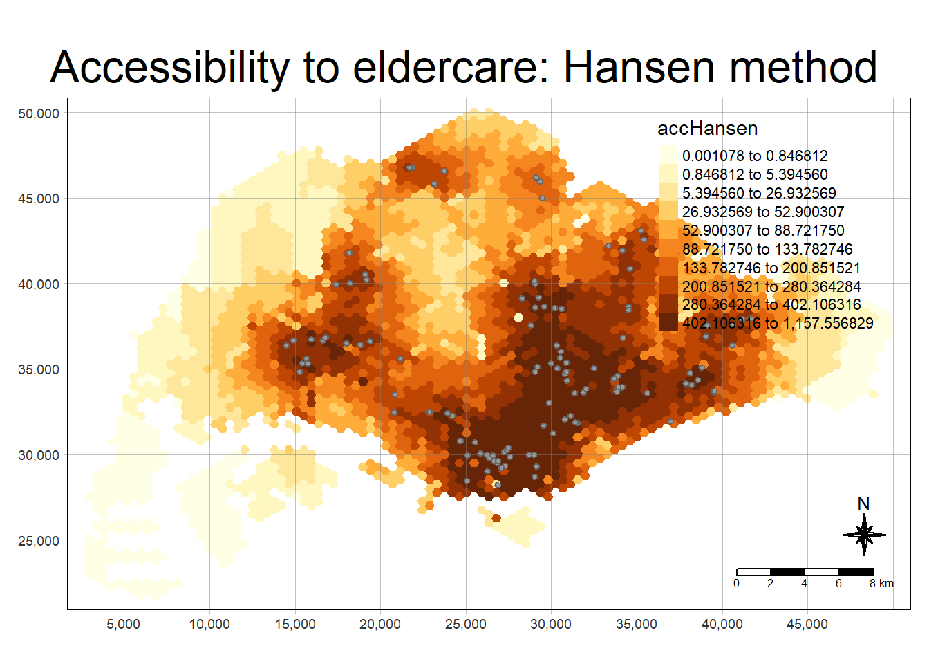
mapex <- st_bbox(hexagons)

The code chunk below uses a collection of mapping fucntions of tmap package to create a high cartographic quality accessibility to eldercare centre in Singapore.

tmap_mode("plot")
tm_shape(hexagon_Hansen,
         bbox = mapex) + 
  tm_fill(col = "accHansen",
          n = 10,
          style = "quantile",
          border.col = "black",
          border.lwd = 1) +
tm_shape(eldercare) +
  tm_symbols(size = 0.1) +
  tm_layout(main.title = "Accessibility to eldercare: Hansen method",
            main.title.position = "center",
            main.title.size = 2,
            legend.outside = FALSE,
            legend.height = 0.45, 
            legend.width = 3.0,
            legend.format = list(digits = 6),
            legend.position = c("right", "top"),
            frame = TRUE) +
  tm_compass(type="8star", size = 2) +
  tm_scale_bar(width = 0.15) +
  tm_grid(lwd = 0.1, alpha = 0.5)