pacman::p_load(olsrr, corrplot, ggpubr, sf, spdep, GWmodel, tmap, tidyverse, gtsummary, readr)In-class Exercise 8: Building hedonic pricing model with gwr
13.5 Geospatial Data Wrangling 13.5.1 Importing geospatial data The geospatial data used in this hands-on exercise is called MP14_SUBZONE_WEB_PL. It is in ESRI shapefile format. The shapefile consists of URA Master Plan 2014’s planning subzone boundaries. Polygon features are used to represent these geographic boundaries. The GIS data is in svy21 projected coordinates systems.
The code chunk below is used to import MP_SUBZONE_WEB_PL shapefile by using st_read() of sf packages.
mpsz = st_read(dsn = "data/Geospatial", layer = "MP14_SUBZONE_WEB_PL")Reading layer `MP14_SUBZONE_WEB_PL' from data source
`C:\Harith-oh\IS415-Harith\In-class_Ex\data\Geospatial' using driver `ESRI Shapefile'
Simple feature collection with 323 features and 15 fields
Geometry type: MULTIPOLYGON
Dimension: XY
Bounding box: xmin: 2667.538 ymin: 15748.72 xmax: 56396.44 ymax: 50256.33
Projected CRS: SVY21Reading layer MP14_SUBZONE_WEB_PL' from data sourceD:gdsa’ using driver `ESRI Shapefile’ Simple feature collection with 323 features and 15 fields Geometry type: MULTIPOLYGON Dimension: XY Bounding box: xmin: 2667.538 ymin: 15748.72 xmax: 56396.44 ymax: 50256.33 Projected CRS: SVY21 The report above shows that the R object used to contain the imported MP14_SUBZONE_WEB_PL shapefile is called mpsz and it is a simple feature object. The geometry type is multipolygon. it is also important to note that mpsz simple feature object does not have EPSG information.
13.5.2 Updating CRS information The code chunk below updates the newly imported mpsz with the correct ESPG code (i.e. 3414)
mpsz_svy21 <- st_transform(mpsz, 3414)After transforming the projection metadata, you can varify the projection of the newly transformed mpsz_svy21 by using st_crs() of sf package.
The code chunk below will be used to varify the newly transformed mpsz_svy21.
st_crs(mpsz_svy21)Coordinate Reference System:
User input: EPSG:3414
wkt:
PROJCRS["SVY21 / Singapore TM",
BASEGEOGCRS["SVY21",
DATUM["SVY21",
ELLIPSOID["WGS 84",6378137,298.257223563,
LENGTHUNIT["metre",1]]],
PRIMEM["Greenwich",0,
ANGLEUNIT["degree",0.0174532925199433]],
ID["EPSG",4757]],
CONVERSION["Singapore Transverse Mercator",
METHOD["Transverse Mercator",
ID["EPSG",9807]],
PARAMETER["Latitude of natural origin",1.36666666666667,
ANGLEUNIT["degree",0.0174532925199433],
ID["EPSG",8801]],
PARAMETER["Longitude of natural origin",103.833333333333,
ANGLEUNIT["degree",0.0174532925199433],
ID["EPSG",8802]],
PARAMETER["Scale factor at natural origin",1,
SCALEUNIT["unity",1],
ID["EPSG",8805]],
PARAMETER["False easting",28001.642,
LENGTHUNIT["metre",1],
ID["EPSG",8806]],
PARAMETER["False northing",38744.572,
LENGTHUNIT["metre",1],
ID["EPSG",8807]]],
CS[Cartesian,2],
AXIS["northing (N)",north,
ORDER[1],
LENGTHUNIT["metre",1]],
AXIS["easting (E)",east,
ORDER[2],
LENGTHUNIT["metre",1]],
USAGE[
SCOPE["Cadastre, engineering survey, topographic mapping."],
AREA["Singapore - onshore and offshore."],
BBOX[1.13,103.59,1.47,104.07]],
ID["EPSG",3414]]Coordinate Reference System: User input: EPSG:3414 wkt: PROJCRS[“SVY21 / Singapore TM”, BASEGEOGCRS[“SVY21”, DATUM[“SVY21”, ELLIPSOID[“WGS 84”,6378137,298.257223563, LENGTHUNIT[“metre”,1]]], PRIMEM[“Greenwich”,0, ANGLEUNIT[“degree”,0.0174532925199433]], ID[“EPSG”,4757]], CONVERSION[“Singapore Transverse Mercator”, METHOD[“Transverse Mercator”, ID[“EPSG”,9807]], PARAMETER[“Latitude of natural origin”,1.36666666666667, ANGLEUNIT[“degree”,0.0174532925199433], ID[“EPSG”,8801]], PARAMETER[“Longitude of natural origin”,103.833333333333, ANGLEUNIT[“degree”,0.0174532925199433], ID[“EPSG”,8802]], PARAMETER[“Scale factor at natural origin”,1, SCALEUNIT[“unity”,1], ID[“EPSG”,8805]], PARAMETER[“False easting”,28001.642, LENGTHUNIT[“metre”,1], ID[“EPSG”,8806]], PARAMETER[“False northing”,38744.572, LENGTHUNIT[“metre”,1], ID[“EPSG”,8807]]], CS[Cartesian,2], AXIS[“northing (N)”,north, ORDER[1], LENGTHUNIT[“metre”,1]], AXIS[“easting (E)”,east, ORDER[2], LENGTHUNIT[“metre”,1]], USAGE[ SCOPE[“Cadastre, engineering survey, topographic mapping.”], AREA[“Singapore - onshore and offshore.”], BBOX[1.13,103.59,1.47,104.07]], ID[“EPSG”,3414]] Notice that the EPSG: is indicated as 3414 now.
Next, you will reveal the extent of mpsz_svy21 by using st_bbox() of sf package.
st_bbox(mpsz_svy21) #view extent xmin ymin xmax ymax
2667.538 15748.721 56396.440 50256.334 xmin ymin xmax ymax 2667.538 15748.721 56396.440 50256.334
13.6 Aspatial Data Wrangling 13.6.1 Importing the aspatial data The condo_resale_2015 is in csv file format. The codes chunk below uses read_csv() function of readr package to import condo_resale_2015 into R as a tibble data frame called condo_resale.
condo_resale = read_csv("data/Aspatial/Condo_resale_2015.csv")After importing the data file into R, it is important for us to examine if the data file has been imported correctly.
The codes chunks below uses glimpse() to display the data structure of will do the job.
glimpse(condo_resale)Rows: 1,436
Columns: 23
$ LATITUDE <dbl> 1.287145, 1.328698, 1.313727, 1.308563, 1.321437,…
$ LONGITUDE <dbl> 103.7802, 103.8123, 103.7971, 103.8247, 103.9505,…
$ POSTCODE <dbl> 118635, 288420, 267833, 258380, 467169, 466472, 3…
$ SELLING_PRICE <dbl> 3000000, 3880000, 3325000, 4250000, 1400000, 1320…
$ AREA_SQM <dbl> 309, 290, 248, 127, 145, 139, 218, 141, 165, 168,…
$ AGE <dbl> 30, 32, 33, 7, 28, 22, 24, 24, 27, 31, 17, 22, 6,…
$ PROX_CBD <dbl> 7.941259, 6.609797, 6.898000, 4.038861, 11.783402…
$ PROX_CHILDCARE <dbl> 0.16597932, 0.28027246, 0.42922669, 0.39473543, 0…
$ PROX_ELDERLYCARE <dbl> 2.5198118, 1.9333338, 0.5021395, 1.9910316, 1.121…
$ PROX_URA_GROWTH_AREA <dbl> 6.618741, 7.505109, 6.463887, 4.906512, 6.410632,…
$ PROX_HAWKER_MARKET <dbl> 1.76542207, 0.54507614, 0.37789301, 1.68259969, 0…
$ PROX_KINDERGARTEN <dbl> 0.05835552, 0.61592412, 0.14120309, 0.38200076, 0…
$ PROX_MRT <dbl> 0.5607188, 0.6584461, 0.3053433, 0.6910183, 0.528…
$ PROX_PARK <dbl> 1.1710446, 0.1992269, 0.2779886, 0.9832843, 0.116…
$ PROX_PRIMARY_SCH <dbl> 1.6340256, 0.9747834, 1.4715016, 1.4546324, 0.709…
$ PROX_TOP_PRIMARY_SCH <dbl> 3.3273195, 0.9747834, 1.4715016, 2.3006394, 0.709…
$ PROX_SHOPPING_MALL <dbl> 2.2102717, 2.9374279, 1.2256850, 0.3525671, 1.307…
$ PROX_SUPERMARKET <dbl> 0.9103958, 0.5900617, 0.4135583, 0.4162219, 0.581…
$ PROX_BUS_STOP <dbl> 0.10336166, 0.28673408, 0.28504777, 0.29872340, 0…
$ NO_Of_UNITS <dbl> 18, 20, 27, 30, 30, 31, 32, 32, 32, 32, 34, 34, 3…
$ FAMILY_FRIENDLY <dbl> 0, 0, 0, 0, 0, 1, 1, 0, 1, 1, 0, 0, 0, 0, 0, 0, 0…
$ FREEHOLD <dbl> 1, 1, 1, 1, 1, 1, 1, 1, 1, 0, 1, 1, 1, 1, 1, 1, 1…
$ LEASEHOLD_99YR <dbl> 0, 0, 0, 0, 0, 0, 0, 0, 0, 0, 0, 0, 0, 0, 0, 0, 0…head(condo_resale$LONGITUDE) #see the data in XCOORD column[1] 103.7802 103.8123 103.7971 103.8247 103.9505 103.9386head(condo_resale$LATITUDE) #see the data in YCOORD column[1] 1.287145 1.328698 1.313727 1.308563 1.321437 1.314198[1] 1.287145 1.328698 1.313727 1.308563 1.321437 1.314198 Next, summary() of base R is used to display the summary statistics of cond_resale tibble data frame.
summary(condo_resale) LATITUDE LONGITUDE POSTCODE SELLING_PRICE
Min. :1.240 Min. :103.7 Min. : 18965 Min. : 540000
1st Qu.:1.309 1st Qu.:103.8 1st Qu.:259849 1st Qu.: 1100000
Median :1.328 Median :103.8 Median :469298 Median : 1383222
Mean :1.334 Mean :103.8 Mean :440439 Mean : 1751211
3rd Qu.:1.357 3rd Qu.:103.9 3rd Qu.:589486 3rd Qu.: 1950000
Max. :1.454 Max. :104.0 Max. :828833 Max. :18000000
AREA_SQM AGE PROX_CBD PROX_CHILDCARE
Min. : 34.0 Min. : 0.00 Min. : 0.3869 Min. :0.004927
1st Qu.:103.0 1st Qu.: 5.00 1st Qu.: 5.5574 1st Qu.:0.174481
Median :121.0 Median :11.00 Median : 9.3567 Median :0.258135
Mean :136.5 Mean :12.14 Mean : 9.3254 Mean :0.326313
3rd Qu.:156.0 3rd Qu.:18.00 3rd Qu.:12.6661 3rd Qu.:0.368293
Max. :619.0 Max. :37.00 Max. :19.1804 Max. :3.465726
PROX_ELDERLYCARE PROX_URA_GROWTH_AREA PROX_HAWKER_MARKET PROX_KINDERGARTEN
Min. :0.05451 Min. :0.2145 Min. :0.05182 Min. :0.004927
1st Qu.:0.61254 1st Qu.:3.1643 1st Qu.:0.55245 1st Qu.:0.276345
Median :0.94179 Median :4.6186 Median :0.90842 Median :0.413385
Mean :1.05351 Mean :4.5981 Mean :1.27987 Mean :0.458903
3rd Qu.:1.35122 3rd Qu.:5.7550 3rd Qu.:1.68578 3rd Qu.:0.578474
Max. :3.94916 Max. :9.1554 Max. :5.37435 Max. :2.229045
PROX_MRT PROX_PARK PROX_PRIMARY_SCH PROX_TOP_PRIMARY_SCH
Min. :0.05278 Min. :0.02906 Min. :0.07711 Min. :0.07711
1st Qu.:0.34646 1st Qu.:0.26211 1st Qu.:0.44024 1st Qu.:1.34451
Median :0.57430 Median :0.39926 Median :0.63505 Median :1.88213
Mean :0.67316 Mean :0.49802 Mean :0.75471 Mean :2.27347
3rd Qu.:0.84844 3rd Qu.:0.65592 3rd Qu.:0.95104 3rd Qu.:2.90954
Max. :3.48037 Max. :2.16105 Max. :3.92899 Max. :6.74819
PROX_SHOPPING_MALL PROX_SUPERMARKET PROX_BUS_STOP NO_Of_UNITS
Min. :0.0000 Min. :0.0000 Min. :0.001595 Min. : 18.0
1st Qu.:0.5258 1st Qu.:0.3695 1st Qu.:0.098356 1st Qu.: 188.8
Median :0.9357 Median :0.5687 Median :0.151710 Median : 360.0
Mean :1.0455 Mean :0.6141 Mean :0.193974 Mean : 409.2
3rd Qu.:1.3994 3rd Qu.:0.7862 3rd Qu.:0.220466 3rd Qu.: 590.0
Max. :3.4774 Max. :2.2441 Max. :2.476639 Max. :1703.0
FAMILY_FRIENDLY FREEHOLD LEASEHOLD_99YR
Min. :0.0000 Min. :0.0000 Min. :0.0000
1st Qu.:0.0000 1st Qu.:0.0000 1st Qu.:0.0000
Median :0.0000 Median :0.0000 Median :0.0000
Mean :0.4868 Mean :0.4227 Mean :0.4882
3rd Qu.:1.0000 3rd Qu.:1.0000 3rd Qu.:1.0000
Max. :1.0000 Max. :1.0000 Max. :1.0000 13.6.2 Converting aspatial data frame into a sf object Currently, the condo_resale tibble data frame is aspatial. We will convert it to a sf object. The code chunk below converts condo_resale data frame into a simple feature data frame by using st_as_sf() of sf packages.
condo_resale.sf <- st_as_sf(condo_resale,
                            coords = c("LONGITUDE", "LATITUDE"),
                            crs=4326) %>%
  st_transform(crs=3414)
Notice that st_transform() of sf package is used to convert the coordinates from wgs84 (i.e. crs:4326) to svy21 (i.e. crs=3414).
Next, head() is used to list the content of condo_resale.sf object.
head(condo_resale.sf)Simple feature collection with 6 features and 21 fields
Geometry type: POINT
Dimension: XY
Bounding box: xmin: 22085.12 ymin: 29951.54 xmax: 41042.56 ymax: 34546.2
Projected CRS: SVY21 / Singapore TM
# A tibble: 6 × 22
POSTCODE SELLI…¹ AREA_…² AGE PROX_…³ PROX_…⁴ PROX_…⁵ PROX_…⁶ PROX_…⁷ PROX_…⁸
<dbl> <dbl> <dbl> <dbl> <dbl> <dbl> <dbl> <dbl> <dbl> <dbl>
1 118635 3000000 309 30 7.94 0.166 2.52 6.62 1.77 0.0584
2 288420 3880000 290 32 6.61 0.280 1.93 7.51 0.545 0.616
3 267833 3325000 248 33 6.90 0.429 0.502 6.46 0.378 0.141
4 258380 4250000 127 7 4.04 0.395 1.99 4.91 1.68 0.382
5 467169 1400000 145 28 11.8 0.119 1.12 6.41 0.565 0.461
6 466472 1320000 139 22 10.3 0.125 0.789 5.09 0.781 0.0994
# … with 12 more variables: PROX_MRT <dbl>, PROX_PARK <dbl>,
# PROX_PRIMARY_SCH <dbl>, PROX_TOP_PRIMARY_SCH <dbl>,
# PROX_SHOPPING_MALL <dbl>, PROX_SUPERMARKET <dbl>, PROX_BUS_STOP <dbl>,
# NO_Of_UNITS <dbl>, FAMILY_FRIENDLY <dbl>, FREEHOLD <dbl>,
# LEASEHOLD_99YR <dbl>, geometry <POINT [m]>, and abbreviated variable names
# ¹SELLING_PRICE, ²AREA_SQM, ³PROX_CBD, ⁴PROX_CHILDCARE, ⁵PROX_ELDERLYCARE,
# ⁶PROX_URA_GROWTH_AREA, ⁷PROX_HAWKER_MARKET, ⁸PROX_KINDERGARTENNotice that the output is in point feature data frame.
corrplot::corrplot(cor(condo_resale[, 5:23]), diag = FALSE, order = "AOE",
         tl.pos = "td", tl.cex = 0.5, method = "number", type = "upper")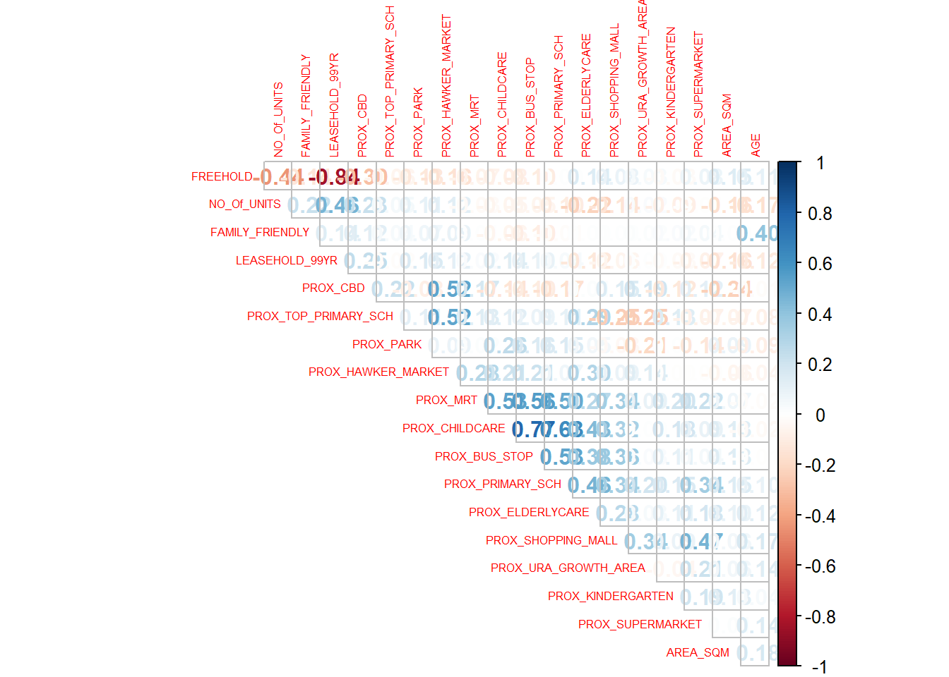
13.7 Exploratory Data Analysis (EDA) In the section, you will learn how to use statistical graphics functions of ggplot2 package to perform EDA.
13.7.1 EDA using statistical graphics We can plot the distribution of SELLING_PRICE by using appropriate Exploratory Data Analysis (EDA) as shown in the code chunk below.
ggplot(data=condo_resale.sf, aes(x=`SELLING_PRICE`)) +
  geom_histogram(bins=20, color="black", fill="light blue")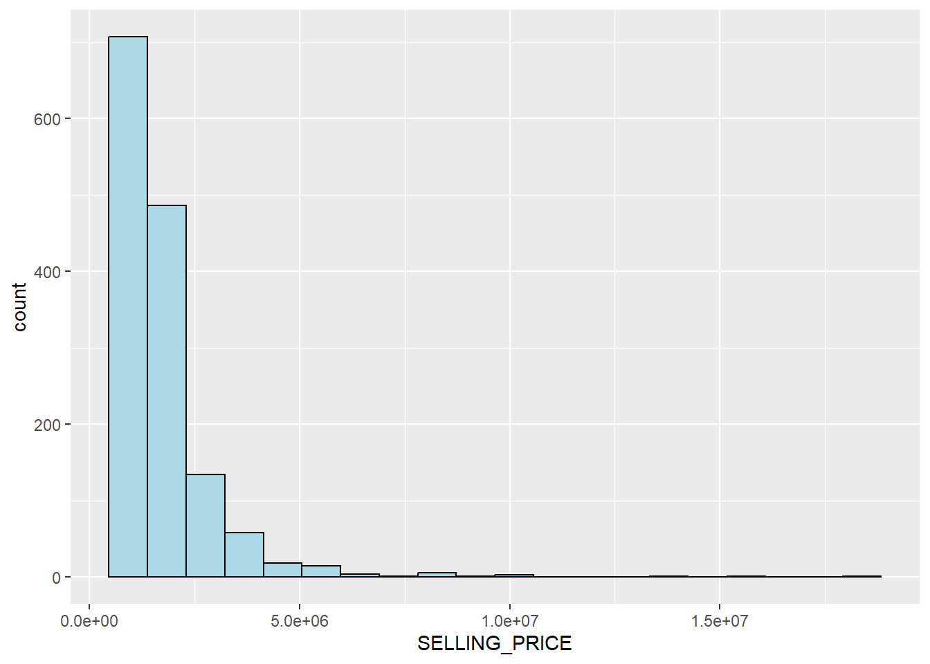
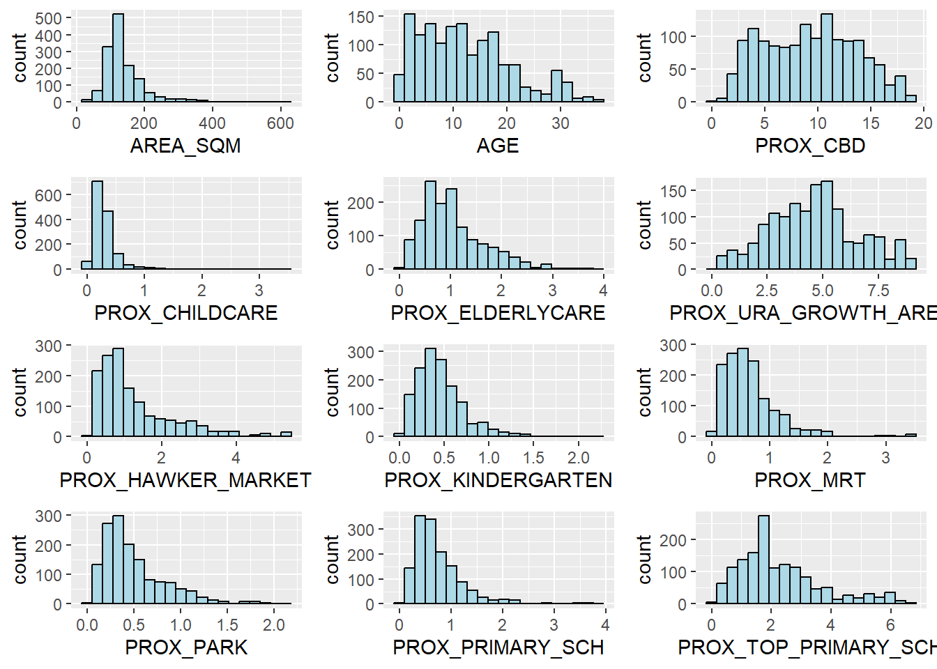
13.7.2 Multiple Histogram Plots distribution of variables In this section, you will learn how to draw a small multiple histograms (also known as trellis plot) by using ggarrange() of ggpubr package.
The code chunk below is used to create 12 histograms. Then, ggarrange() is used to organised these histogram into a 3 columns by 4 rows small multiple plot.
AREA_SQM <- ggplot(data=condo_resale.sf, aes(x= `AREA_SQM`)) +
  geom_histogram(bins=20, color="black", fill="light blue")

AGE <- ggplot(data=condo_resale.sf, aes(x= `AGE`)) +
  geom_histogram(bins=20, color="black", fill="light blue")

PROX_CBD <- ggplot(data=condo_resale.sf, aes(x= `PROX_CBD`)) +
  geom_histogram(bins=20, color="black", fill="light blue")

PROX_CHILDCARE <- ggplot(data=condo_resale.sf, aes(x= `PROX_CHILDCARE`)) +
  geom_histogram(bins=20, color="black", fill="light blue")

PROX_ELDERLYCARE <- ggplot(data=condo_resale.sf, aes(x= `PROX_ELDERLYCARE`)) +
  geom_histogram(bins=20, color="black", fill="light blue")

PROX_URA_GROWTH_AREA <- ggplot(data=condo_resale.sf,
                               aes(x= `PROX_URA_GROWTH_AREA`)) +
  geom_histogram(bins=20, color="black", fill="light blue")

PROX_HAWKER_MARKET <- ggplot(data=condo_resale.sf, aes(x= `PROX_HAWKER_MARKET`)) +
  geom_histogram(bins=20, color="black", fill="light blue")

PROX_KINDERGARTEN <- ggplot(data=condo_resale.sf, aes(x= `PROX_KINDERGARTEN`)) +
  geom_histogram(bins=20, color="black", fill="light blue")

PROX_MRT <- ggplot(data=condo_resale.sf, aes(x= `PROX_MRT`)) +
  geom_histogram(bins=20, color="black", fill="light blue")

PROX_PARK <- ggplot(data=condo_resale.sf, aes(x= `PROX_PARK`)) +
  geom_histogram(bins=20, color="black", fill="light blue")

PROX_PRIMARY_SCH <- ggplot(data=condo_resale.sf, aes(x= `PROX_PRIMARY_SCH`)) +
  geom_histogram(bins=20, color="black", fill="light blue")

PROX_TOP_PRIMARY_SCH <- ggplot(data=condo_resale.sf,
                               aes(x= `PROX_TOP_PRIMARY_SCH`)) +
  geom_histogram(bins=20, color="black", fill="light blue")

ggarrange(AREA_SQM, AGE, PROX_CBD, PROX_CHILDCARE, PROX_ELDERLYCARE,
          PROX_URA_GROWTH_AREA, PROX_HAWKER_MARKET, PROX_KINDERGARTEN, PROX_MRT,
          PROX_PARK, PROX_PRIMARY_SCH, PROX_TOP_PRIMARY_SCH,
          ncol = 3, nrow = 4)