if (!require('pacman', character.only = T)){
install.packages('pacman')
}
library('pacman')Take-home Exercise 1
1 Introduction
This study aims to analyse the geographical distribution of functional and non-function water points and their co-locations if any in Osun State, Nigeria by applying appropriate spatial point patterns analysis methods.
- To address the issue of providing a clean and sustainable water supply to the rural community, a global Water Point Data Exchange (WPdx) project has been initiated. The main aim of this initiative is to collect water point-related data from rural areas at the water point or small water scheme level and share the data via WPdx Data Repository, a cloud-based data library.
2 Data
The following data sets will be used in the analysis.
Aspatial Data:
For the purpose of this assignment, data from WPdx Global Data Repositories will be used. There are two versions of the data. They are: WPdx-Basic and WPdx+. You are required to use WPdx+ data set.
Geospatial Data:
This study will focus of Osun State, Nigeria. The state boundary GIS data of Nigeria can be downloaded either from The Humanitarian Data Exchange portal or geoBoundaries.
| Data | Format | Description | Source |
|---|---|---|---|
| Nigeria Level-2 Administrative Boundary | Shapefile | Humanitarian Data Exchange(data.humdata.org) or geoBoundaries (geoboundaries.org) |
|
| WPdx Global Data Repositories (WPdx+) | CSV | waterpointdata.org |
3 Install and load packages
Firstly, the code below will check if pacman has been installed. If it has not been installed, R will download and install it, before activating it for use during this session.
To get started, the following packages will be used for this exercise:
tidyverse, funModeling, maptools, sf, raster, spatstat & tmap.
pacman::p_load(maptools, sf, tidyverse, raster, spatstat, tmap, sfdep, funModeling)4 Import Data
Importing & examining the contents of each data set.
4.1 Importing geoBoundaries Nigeria Level-2 Administrative Boundary Dataset
nigeria = st_read(dsn = "data/Geospatial", layer = "nga_admbnda_adm2_osgof_20190417")Reading layer `nga_admbnda_adm2_osgof_20190417' from data source
`C:\Harith-oh\IS415-Harith\Take-home_Ex\Take-home_Ex01\data\Geospatial'
using driver `ESRI Shapefile'
Simple feature collection with 774 features and 16 fields
Geometry type: MULTIPOLYGON
Dimension: XY
Bounding box: xmin: 2.668534 ymin: 4.273007 xmax: 14.67882 ymax: 13.89442
Geodetic CRS: WGS 84Check CRS
st_crs(nigeria)Coordinate Reference System:
User input: WGS 84
wkt:
GEOGCRS["WGS 84",
DATUM["World Geodetic System 1984",
ELLIPSOID["WGS 84",6378137,298.257223563,
LENGTHUNIT["metre",1]]],
PRIMEM["Greenwich",0,
ANGLEUNIT["degree",0.0174532925199433]],
CS[ellipsoidal,2],
AXIS["latitude",north,
ORDER[1],
ANGLEUNIT["degree",0.0174532925199433]],
AXIS["longitude",east,
ORDER[2],
ANGLEUNIT["degree",0.0174532925199433]],
ID["EPSG",4326]]4.2 Converting the Coordinating Reference System
In the code below, we will convert the Geographic Coordinate Reference System from WGS84 to EPSG:26391 Projected Coordinate System.
nigeria26391 <- st_transform(nigeria, crs = 26391)st_crs(nigeria26391)Coordinate Reference System:
User input: EPSG:26391
wkt:
PROJCRS["Minna / Nigeria West Belt",
BASEGEOGCRS["Minna",
DATUM["Minna",
ELLIPSOID["Clarke 1880 (RGS)",6378249.145,293.465,
LENGTHUNIT["metre",1]]],
PRIMEM["Greenwich",0,
ANGLEUNIT["degree",0.0174532925199433]],
ID["EPSG",4263]],
CONVERSION["Nigeria West Belt",
METHOD["Transverse Mercator",
ID["EPSG",9807]],
PARAMETER["Latitude of natural origin",4,
ANGLEUNIT["degree",0.0174532925199433],
ID["EPSG",8801]],
PARAMETER["Longitude of natural origin",4.5,
ANGLEUNIT["degree",0.0174532925199433],
ID["EPSG",8802]],
PARAMETER["Scale factor at natural origin",0.99975,
SCALEUNIT["unity",1],
ID["EPSG",8805]],
PARAMETER["False easting",230738.26,
LENGTHUNIT["metre",1],
ID["EPSG",8806]],
PARAMETER["False northing",0,
LENGTHUNIT["metre",1],
ID["EPSG",8807]]],
CS[Cartesian,2],
AXIS["(E)",east,
ORDER[1],
LENGTHUNIT["metre",1]],
AXIS["(N)",north,
ORDER[2],
LENGTHUNIT["metre",1]],
USAGE[
SCOPE["Engineering survey, topographic mapping."],
AREA["Nigeria - onshore west of 6°30'E, onshore and offshore shelf."],
BBOX[3.57,2.69,13.9,6.5]],
ID["EPSG",26391]]After running the code, we can confirm that the data frame has been converted to EPSG:26391 Projected Coordinate System.
4.3 Importing WPdx + Aspatial Data
Since WPdx+ data set is in csv format, we will use read_csv() of readr package to import Water_Point_Data_Exchange_-_PlusWPdx.csv and output it to an R object called wpdx.
wpdx <- read_csv("data/Aspatial/Water_Point_Data_Exchange.csv") %>% filter(`#clean_country_name` == "Nigeria")list(wpdx)[[1]]
# A tibble: 95,008 × 70
row_id `#source` #lat_…¹ #lon_…² #repo…³ #stat…⁴ #wate…⁵ #wate…⁶ #wate…⁷
<dbl> <chr> <dbl> <dbl> <chr> <chr> <chr> <chr> <chr>
1 429068 GRID3 7.98 5.12 08/29/… Unknown <NA> <NA> Tapsta…
2 222071 Federal Minis… 6.96 3.60 08/16/… Yes Boreho… Well Mechan…
3 160612 WaterAid 6.49 7.93 12/04/… Yes Boreho… Well Hand P…
4 160669 WaterAid 6.73 7.65 12/04/… Yes Boreho… Well <NA>
5 160642 WaterAid 6.78 7.66 12/04/… Yes Boreho… Well Hand P…
6 160628 WaterAid 6.96 7.78 12/04/… Yes Boreho… Well Hand P…
7 160632 WaterAid 7.02 7.84 12/04/… Yes Boreho… Well Hand P…
8 642747 Living Water … 7.33 8.98 10/03/… Yes Boreho… Well Mechan…
9 642456 Living Water … 7.17 9.11 10/03/… Yes Boreho… Well Hand P…
10 641347 Living Water … 7.20 9.22 03/28/… Yes Boreho… Well Hand P…
# … with 94,998 more rows, 61 more variables: `#water_tech_category` <chr>,
# `#facility_type` <chr>, `#clean_country_name` <chr>, `#clean_adm1` <chr>,
# `#clean_adm2` <chr>, `#clean_adm3` <chr>, `#clean_adm4` <chr>,
# `#install_year` <dbl>, `#installer` <chr>, `#rehab_year` <lgl>,
# `#rehabilitator` <lgl>, `#management_clean` <chr>, `#status_clean` <chr>,
# `#pay` <chr>, `#fecal_coliform_presence` <chr>,
# `#fecal_coliform_value` <dbl>, `#subjective_quality` <chr>, …Our output shows our wpdx tibble data frame consists of 97,478 rows and 74 columns. The useful fields we would be paying attention to is the #lat_deg and #lon_deg columns, which are in the decimal degree format. By viewing the Data Standard on wpdx’s website, we know that the latitude and longitude is in the wgs84 Geographic Coordinate System.
4.3.1 Creating a simple data frame from an Aspatial Data Frame
As the geometry is available in wkt in the column New Georeferenced Column, we can use st_as_sfc() to import the geomtry
wpdx$Geometry <- st_as_sfc(wpdx$`New Georeferenced Column`)As there is no spatial data information, firstly, we assign the original projection when converting the tibble dataframe to sf. The original is wgs84 which is EPSG:4326.
wpdx_sf <- st_sf(wpdx, crs=4326)
wpdx_sfSimple feature collection with 95008 features and 70 fields
Geometry type: POINT
Dimension: XY
Bounding box: xmin: 2.707441 ymin: 4.301812 xmax: 14.21828 ymax: 13.86568
Geodetic CRS: WGS 84
# A tibble: 95,008 × 71
row_id `#source` #lat_…¹ #lon_…² #repo…³ #stat…⁴ #wate…⁵ #wate…⁶ #wate…⁷
* <dbl> <chr> <dbl> <dbl> <chr> <chr> <chr> <chr> <chr>
1 429068 GRID3 7.98 5.12 08/29/… Unknown <NA> <NA> Tapsta…
2 222071 Federal Minis… 6.96 3.60 08/16/… Yes Boreho… Well Mechan…
3 160612 WaterAid 6.49 7.93 12/04/… Yes Boreho… Well Hand P…
4 160669 WaterAid 6.73 7.65 12/04/… Yes Boreho… Well <NA>
5 160642 WaterAid 6.78 7.66 12/04/… Yes Boreho… Well Hand P…
6 160628 WaterAid 6.96 7.78 12/04/… Yes Boreho… Well Hand P…
7 160632 WaterAid 7.02 7.84 12/04/… Yes Boreho… Well Hand P…
8 642747 Living Water … 7.33 8.98 10/03/… Yes Boreho… Well Mechan…
9 642456 Living Water … 7.17 9.11 10/03/… Yes Boreho… Well Hand P…
10 641347 Living Water … 7.20 9.22 03/28/… Yes Boreho… Well Hand P…
# … with 94,998 more rows, 62 more variables: `#water_tech_category` <chr>,
# `#facility_type` <chr>, `#clean_country_name` <chr>, `#clean_adm1` <chr>,
# `#clean_adm2` <chr>, `#clean_adm3` <chr>, `#clean_adm4` <chr>,
# `#install_year` <dbl>, `#installer` <chr>, `#rehab_year` <lgl>,
# `#rehabilitator` <lgl>, `#management_clean` <chr>, `#status_clean` <chr>,
# `#pay` <chr>, `#fecal_coliform_presence` <chr>,
# `#fecal_coliform_value` <dbl>, `#subjective_quality` <chr>, …Next, we then convert the projection to the appropriate decimal based projection system.
wpdx_sf <- wpdx_sf %>%
st_transform(crs = 26391)wpdx_spdf <- as_Spatial(wpdx_sf)
wpdx_spdfclass : SpatialPointsDataFrame
features : 95008
extent : 32536.82, 1292096, 33461.24, 1091052 (xmin, xmax, ymin, ymax)
crs : +proj=tmerc +lat_0=4 +lon_0=4.5 +k=0.99975 +x_0=230738.26 +y_0=0 +a=6378249.145 +rf=293.465 +towgs84=-92,-93,122,0,0,0,0 +units=m +no_defs
variables : 70
names : row_id, X.source, X.lat_deg, X.lon_deg, X.report_date, X.status_id, X.water_source_clean, X.water_source_category, X.water_tech_clean, X.water_tech_category, X.facility_type, X.clean_country_name, X.clean_adm1, X.clean_adm2, X.clean_adm3, ...
min values : 10732, Federal Ministry of Water Resources, Nigeria, 4.3018117, 2.707441, 01/01/2010 12:00:00 AM, No, Borehole, Piped Water, Hand Pump, Hand Pump, Improved, Nigeria, Abia, Aba North, NA, ...
max values : 681838, WaterAid UK, 13.865675, 14.2182849, 12/31/2014 12:00:00 AM, Yes, Protected Well, Well, Tapstand, Tapstand, Improved, Nigeria, Zamfara, Zuru, NA, ... 5 Data wrangling
Pre-process and prepare data for analysis.
5.1 Geospatial Data Cleaning
As the wpdx sf dataframe consist of many redundant field, we use select() to select the fields which we want to retain.
nigeria26391 <- nigeria26391 %>%
dplyr::select(c(3:4, 8:9))5.2 Checking for Duplicate Name
nigeria26391$ADM2_EN[duplicated(nigeria26391$ADM2_EN) == TRUE][1] "Bassa" "Ifelodun" "Irepodun" "Nasarawa" "Obi" "Surulere"To reduce duplication of LGA names, we will put the state names behind to make it more specific.
nigeria26391$ADM2_EN[94] <- "Bassa, Kogi"
nigeria26391$ADM2_EN[95] <- "Bassa, Plateau"
nigeria26391$ADM2_EN[304] <- "Ifelodun, Kwara"
nigeria26391$ADM2_EN[305] <- "Ifelodun, Osun"
nigeria26391$ADM2_EN[355] <- "Irepodun, Kwara"
nigeria26391$ADM2_EN[356] <- "Ireopodun, Osun"
nigeria26391$ADM2_EN[519] <- "Nasarawa, Kano"
nigeria26391$ADM2_EN[520] <- "Nasarawa, Nasarawa"
nigeria26391$ADM2_EN[546] <- "Obi, Benue"
nigeria26391$ADM2_EN[547] <- "Obi, Nasarawa"
nigeria26391$ADM2_EN[693] <- "Surulere, Lagos"
nigeria26391$ADM2_EN[694] <- "Surulere, Oyo"To check if the duplication has been resolved.
nigeria26391$ADM2_EN[duplicated(nigeria26391$ADM2_EN) == TRUE]character(0)6 Data Wrangling for Water Point Data
6.1 Understanding Field Names
First, let us have a look at the #status_clean column which stores the information about Functional and Non-Functional data points. The code below returns all values that were used in the column.
freq(data = wpdx_sf,
input = '#status_clean')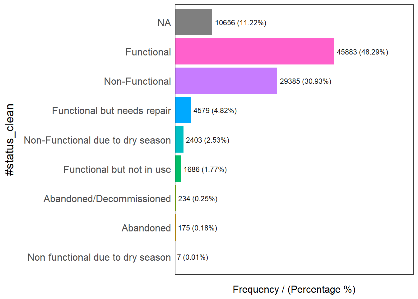
#status_clean frequency percentage cumulative_perc
1 Functional 45883 48.29 48.29
2 Non-Functional 29385 30.93 79.22
3 <NA> 10656 11.22 90.44
4 Functional but needs repair 4579 4.82 95.26
5 Non-Functional due to dry season 2403 2.53 97.79
6 Functional but not in use 1686 1.77 99.56
7 Abandoned/Decommissioned 234 0.25 99.81
8 Abandoned 175 0.18 99.99
9 Non functional due to dry season 7 0.01 100.00As there might be issues performing mathematical calculations with NA labels, we will rename them to unknown.
The code below renames the column #status_clean to status_clean, select only the status_clean for manipulation and then replace all na values to unknown.
wpdx_sf_nga <- wpdx_sf %>%
rename(status_clean = '#status_clean') %>%
dplyr::select(status_clean) %>%
mutate(status_clean = replace_na(status_clean, "unknown"))6.2 ing Data
With our previous knowledge, we can the data to obtain functional proportion counts in each LGA level. We will the wpdx_sf_nga dataframes to option functional and non-functional water points.
wpdx_func <- wpdx_sf_nga %>%
filter(status_clean %in%
c("Functional",
"Functional but not in use",
"Functional but needs repair"))
wpdx_nonfunc <- wpdx_sf_nga %>%
filter(status_clean %in%
c("Abadoned/Decommissioned",
"Abandoned",
"Non-Functional due to dry season",
"Non-Functional",
"Non functional due to dry season"))
wpdx_unknown <- wpdx_sf_nga %>%
filter(status_clean == "unknown")6.3 Point-in-polygon Count
Utilising st_intersects() of sf package and lengths, we check where each data point for the water point which fall inside each LGA. We do each calculation separation so we can cross check later to ensure all the values sum to the same total.
nigeria_wp <- nigeria26391 %>%
mutate(`total_wp` = lengths(
st_intersects(nigeria26391, wpdx_sf_nga))) %>%
mutate(`wp_functional` = lengths(
st_intersects(nigeria26391, wpdx_func))) %>%
mutate(`wp_nonfunctional` = lengths(
st_intersects(nigeria26391, wpdx_nonfunc))) %>%
mutate(`wp_unknown` = lengths(
st_intersects(nigeria26391, wpdx_unknown)))6.4 Saving the Analytical Data in rds format
In order to retain the sf data structure for subsequent analysis, we should save the sf dataframe into rds format.
write_rds(nigeria_wp, "Data/rds/nigeria_wp.rds")6.5 Plotting the Distribution of Total Water Points by LGA in Histogram
Next, we will use mutate() of dplyr package to compute the proportion of Functional and Non- water points.
This is given by Functional Proportion = Functional Count / Total Count.
ggplot(data = nigeria_wp,
aes(x = total_wp)) +
geom_histogram(bins = 20,
color = "black",
fill = "light blue") +
geom_vline(aes(xintercept = mean(
total_wp, na.rm = T)),
color = "red",
linetype = "dashed",
size = 0.8) +
ggtitle("Distribution of total water points by LGA") +
xlab("No. of water points") +
ylab("No of\nLGAs") +
theme(axis.title.y = element_text(angle = 0))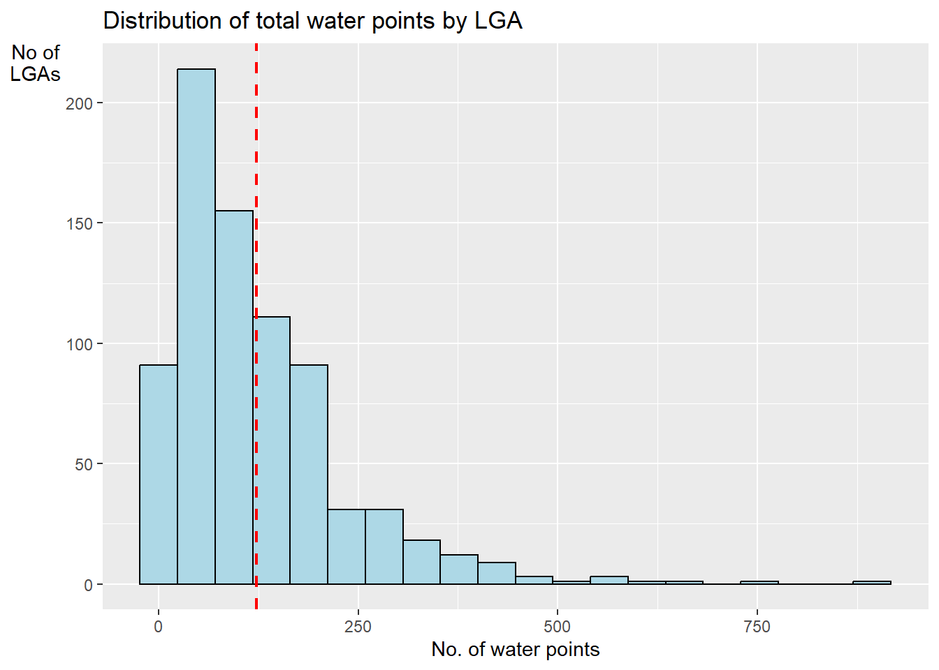
7 Exploratory Spatial Data Analysis (ESDA)
7.1 Import the data saved in rds
We want to import the sf dataframe we have cleaned and prepared earlier
NGA_wp <- read_rds("Data/rds/nigeria_wp.rds")7.2 Visualising Distribution of Non-Functional Water Points
Here, we will plot 2 maps, p1 which shows the functional water points and p2 by total number of water points for side-by-side visualization.
p1 <- tm_shape(NGA_wp) +
tm_fill("wp_functional",
n = 10,
style = "equal",
palette = "Blues") +
tm_borders(lwd = 0.1,
alpha = 1) +
tm_layout(main.title = "Distribution of functional water points by LGA",
legend.outside = FALSE)p2 <- tm_shape(NGA_wp) +
tm_fill("total_wp",
n = 10,
style = "equal",
palette = "Blues") +
tm_borders(lwd = 0.1,
alpha = 1) +
tm_layout(main.title = "Distribution of total water points by LGA",
legend.outside = FALSE)tmap_arrange(p2, p1, nrow = 1)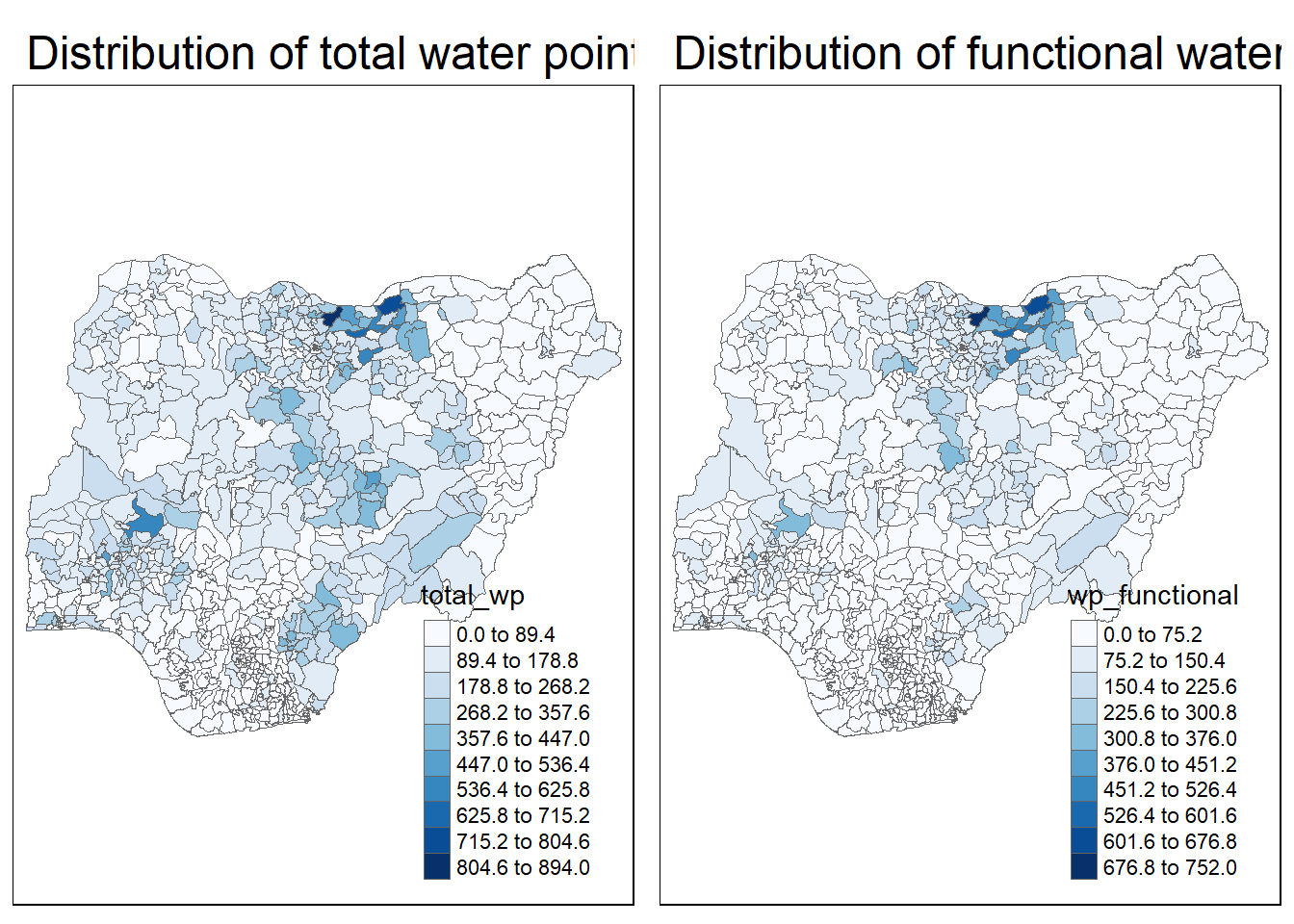
8 Visualising the sf layers
It is to ensure that they have been imported properly and been projected on an appropriate projection system.
tmap_mode("view")
tm_shape(NGA_wp) +
tm_polygons() +
tm_dots()NGA <- as_Spatial(NGA_wp)wpdx_sp <- as(wpdx_spdf, "SpatialPoints")
NGA_sp <- as(NGA, "SpatialPolygons")osun = NGA[NGA@data$ADM1_EN == "Osun",]To plot
plot(osun, main = "Osun")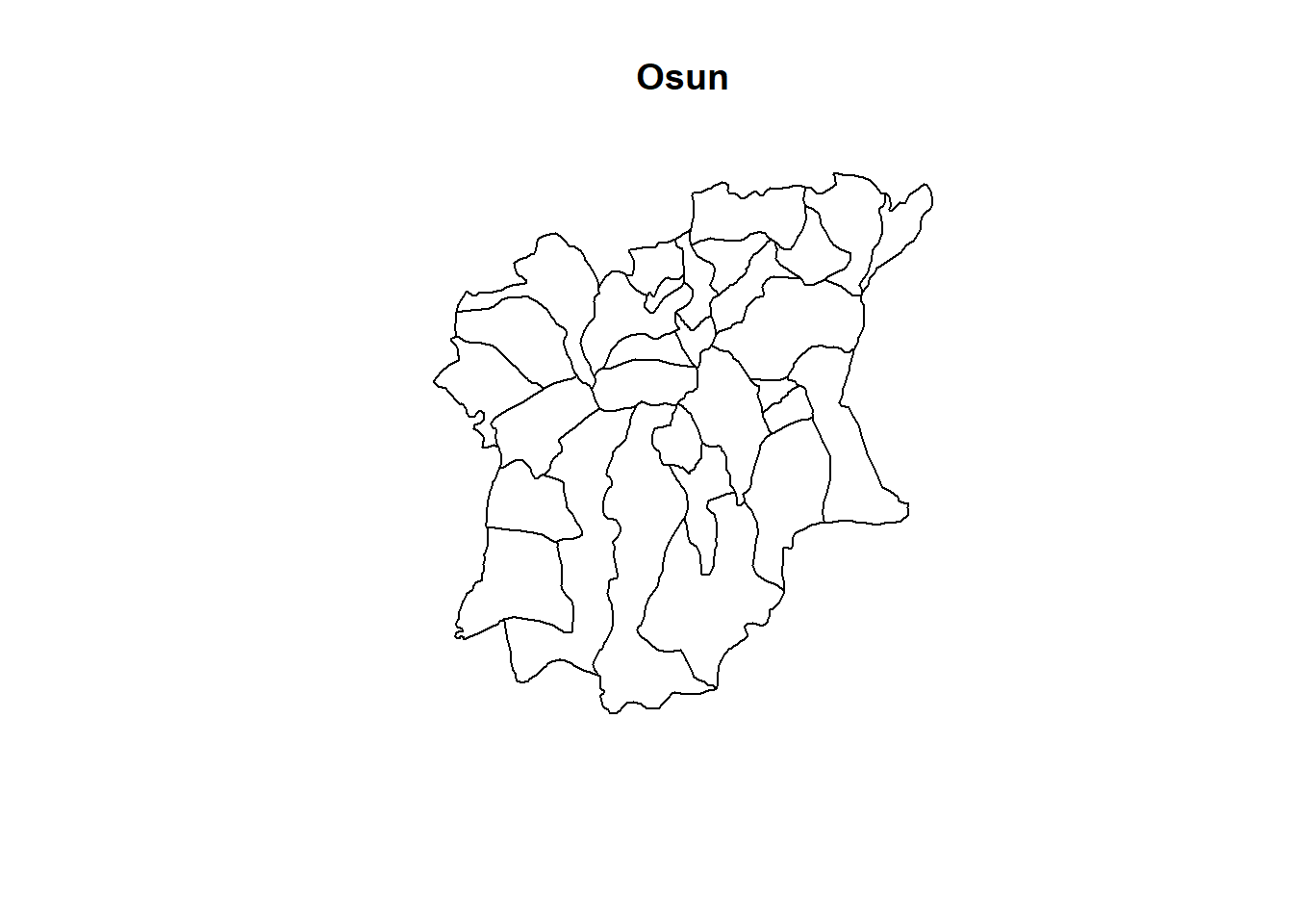
Next, conversion of SpatialPolygonsDataFrame layers into generic spatialpolygons layers
osun_sp = as(osun, "SpatialPolygons")Creating owin object to convert the above spatialpolygons objects into owin objects that is required by spatstat
osun_owin = as(osun_sp, "owin")8.2 Converting the generic sp format into spatstat’s ppp format
Now, we will use as.ppp() function of spatstat to convert the spatial data into spatstat’s ppp object format.
wpdx_ppp <- as(wpdx_sp, "ppp")
wpdx_pppPlanar point pattern: 95008 points
window: rectangle = [32536.8, 1292096.3] x [33461.2, 1091051.6] unitssummary(wpdx_ppp)Planar point pattern: 95008 points
Average intensity 7.132208e-08 points per square unit
Coordinates are given to 2 decimal places
i.e. rounded to the nearest multiple of 0.01 units
Window: rectangle = [32536.8, 1292096.3] x [33461.2, 1091051.6] units
(1260000 x 1058000 units)
Window area = 1.3321e+12 square unitsany(duplicated(wpdx_ppp))[1] FALSE8.3 Combining osun water points
nigeria_osun_PPP = wpdx_ppp[osun_owin]rescale() function is used to transform the unit of measurement from metre to kilometre
nigeria_osun_PPP.km = rescale(nigeria_osun_PPP, 1000, "km")Plotting the Osun water point study area
plot(nigeria_osun_PPP.km, main = "Osun")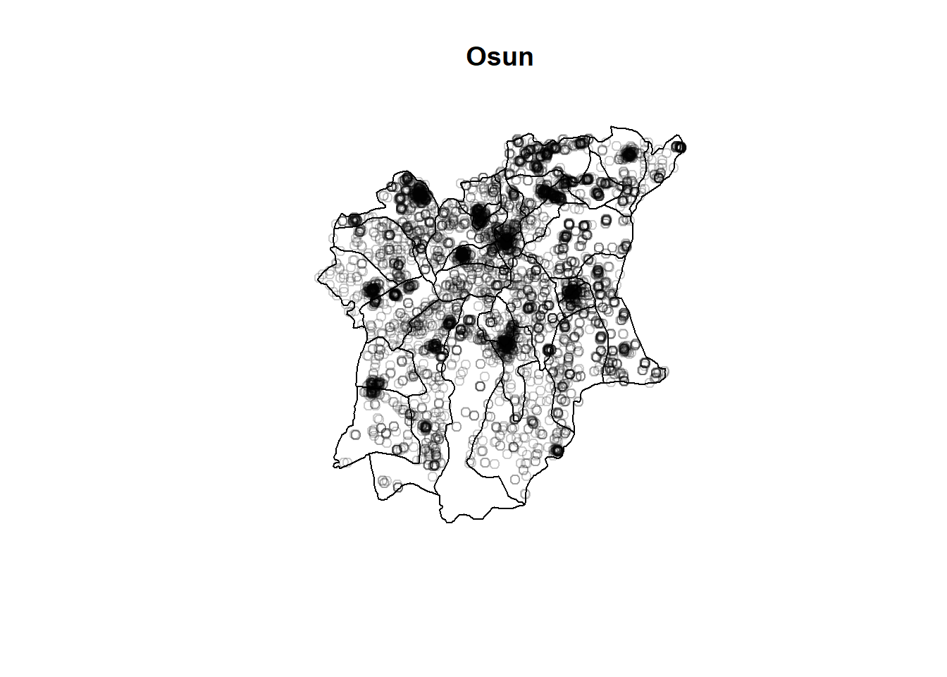
Visualising the SF layer for Osun
tmap_mode("view")
tm_shape(osun) +
tm_polygons() +
tm_dots(size = 0.01,
border.col = "black",
border.lwd = 0.5)9.1 Computing KDE of Osun State
The code below will be used to compute the KDE of Osun. bw.diggle method is used to derive the bandwidth
plot(density(nigeria_osun_PPP.km,
sigma=bw.diggle,
edge=TRUE,
kernel="gaussian"),
main="Osun")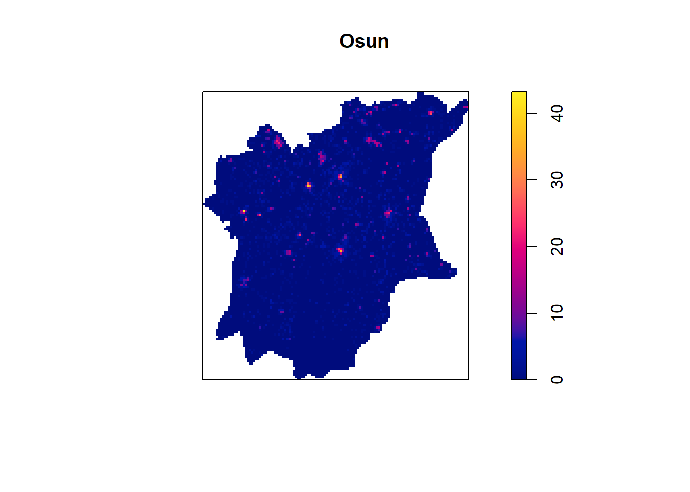
Computing fixed bandwidth KDE
plot(density(nigeria_osun_PPP.km,
sigma=0.25,
edge=TRUE,
kernel="gaussian"),
main="Osun")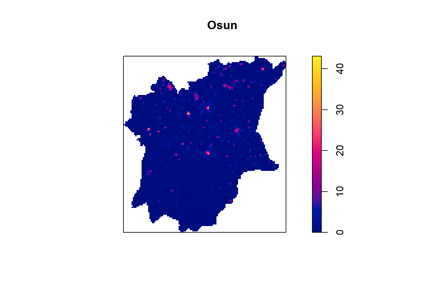
The advantage of kernel density map over point map is that it spreads the known quantity in color shades of waterpoints for each location in Osun State of Nigeria. Whereas for Kernel point, it only provides the pointer of waterpoints for each location in Osun State and does not state the number unless clicked.
wpdx_ppp <- as(wpdx_sp, "ppp")
wpdx_pppPlanar point pattern: 95008 points
window: rectangle = [32536.8, 1292096.3] x [33461.2, 1091051.6] unitssummary(wpdx_ppp)Planar point pattern: 95008 points
Average intensity 7.132208e-08 points per square unit
Coordinates are given to 2 decimal places
i.e. rounded to the nearest multiple of 0.01 units
Window: rectangle = [32536.8, 1292096.3] x [33461.2, 1091051.6] units
(1260000 x 1058000 units)
Window area = 1.3321e+12 square unitsany(duplicated(wpdx_ppp))[1] FALSEosun1 <- tm_shape(osun) +
tm_fill("wp_functional",
n = 10,
style = "equal",
palette = "Blues") +
tm_borders(lwd = 0.1,
alpha = 1) +
tm_layout(main.title = "Distribution of functional water points by LGA",
legend.outside = FALSE)osun2 <- tm_shape(osun) +
tm_fill("wp_nonfunctional",
n = 10,
style = "equal",
palette = "Blues") +
tm_borders(lwd = 0.1,
alpha = 1) +
tm_layout(main.title = "Distribution of total water points by LGA",
legend.outside = FALSE)tmap_arrange(osun2, osun1, nrow = 1)kde_osun_bw <- density(nigeria_osun_PPP,
sigma=bw.diggle,
edge=TRUE,
kernel="gaussian") plot(kde_osun_bw)
osun_bw <- bw.diggle(nigeria_osun_PPP)
osun_bw sigma
217.8511 osun_PPP.km <- rescale(nigeria_osun_PPP, 1000, "km")kde_osun_PPP.bw <- density(nigeria_osun_PPP.km, sigma1=bw.diggle, edge=TRUE, kernel="gaussian")
plot(kde_osun_PPP.bw)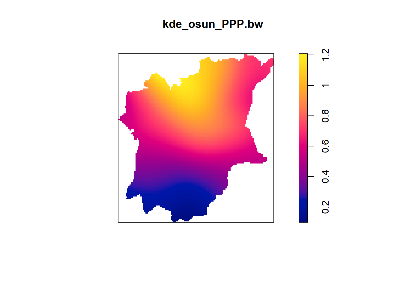
10 Second Spatial Point Analysis
10.1 Performing Clarks Evans Test of Osun State
In this section, we will perform the Clark-Evans test of aggregation for a spatial point pattern by using clarkevans.test() of statspat.
The test hypotheses are:
Ho = The distribution of waterpoints are randomly distributed.
H1= The distribution of waterpoints are not randomly distributed.
The 95% confidence interval will be used.
clarkevans.test(nigeria_osun_PPP,
correction="none",
clipregion=NULL,
alternative=c("two.sided"),
nsim=999)
Clark-Evans test
No edge correction
Monte Carlo test based on 999 simulations of CSR with fixed n
data: nigeria_osun_PPP
R = 0.42836, p-value = 0.002
alternative hypothesis: two-sidedGiven the p value of 0.002 which is lesser than 0.05 of 95% confidence interval, we can conclude that the null hypothesis (H0) should be rejected and the distribution of waterpoints are not randomly distributed.
10.2 Analysing Second Spatial Point using L function
In this section, second spatial point L-function will be using Lest() of spatstat package. Monta carlo simulation test will be used using envelope() of spatstat package.
10.2.1 Computing L Function Estimation
#L_ck = Lest(nigeria_osun_PPP, correction = "Ripley")
#plot(L_ck, . -r ~ r,
# ylab= "L(d)-r", xlab = "d(m)")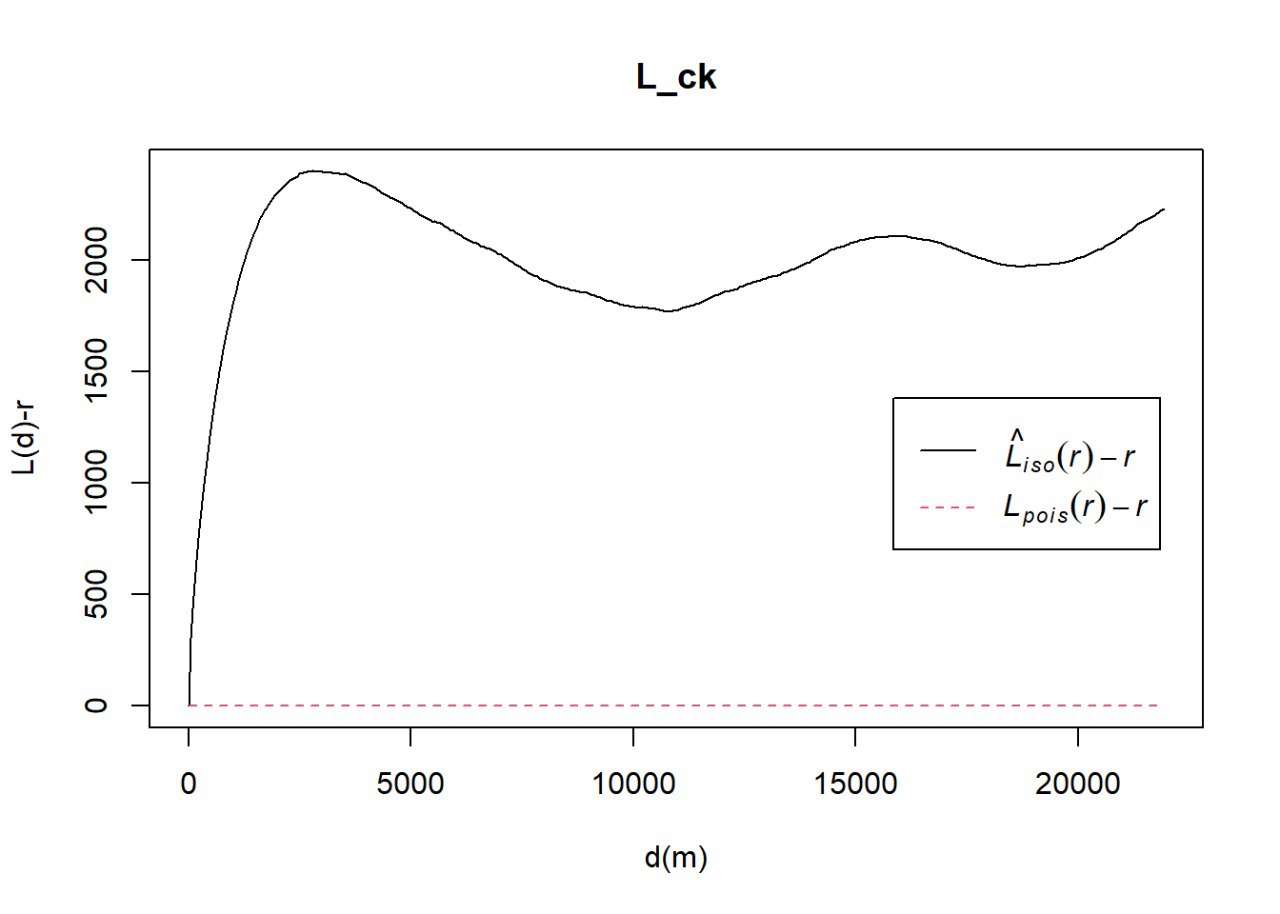
10.2.2 Performing Complete Spatial Random Test
To confirm the observed spatial patterns above, a hypothesis test will be conducted. The hypothesis and test are as follows:
Ho = The distribution of Water Point at Osun State are randomly distributed.
H1= The distribution of Water Point at Osun State are not randomly distributed.
The null hypothesis will be rejected if p-value if smaller than alpha value of 0.001.
The code chunk below is used to perform the hypothesis testing
#L_ck.csr <- envelope(nigeria_osun_PPP, Lest, nsim = 39, rank = 1, glocal=TRUE)#plot(L_ck.csr, . - r ~ r, xlab="d", ylab="L(d)-r")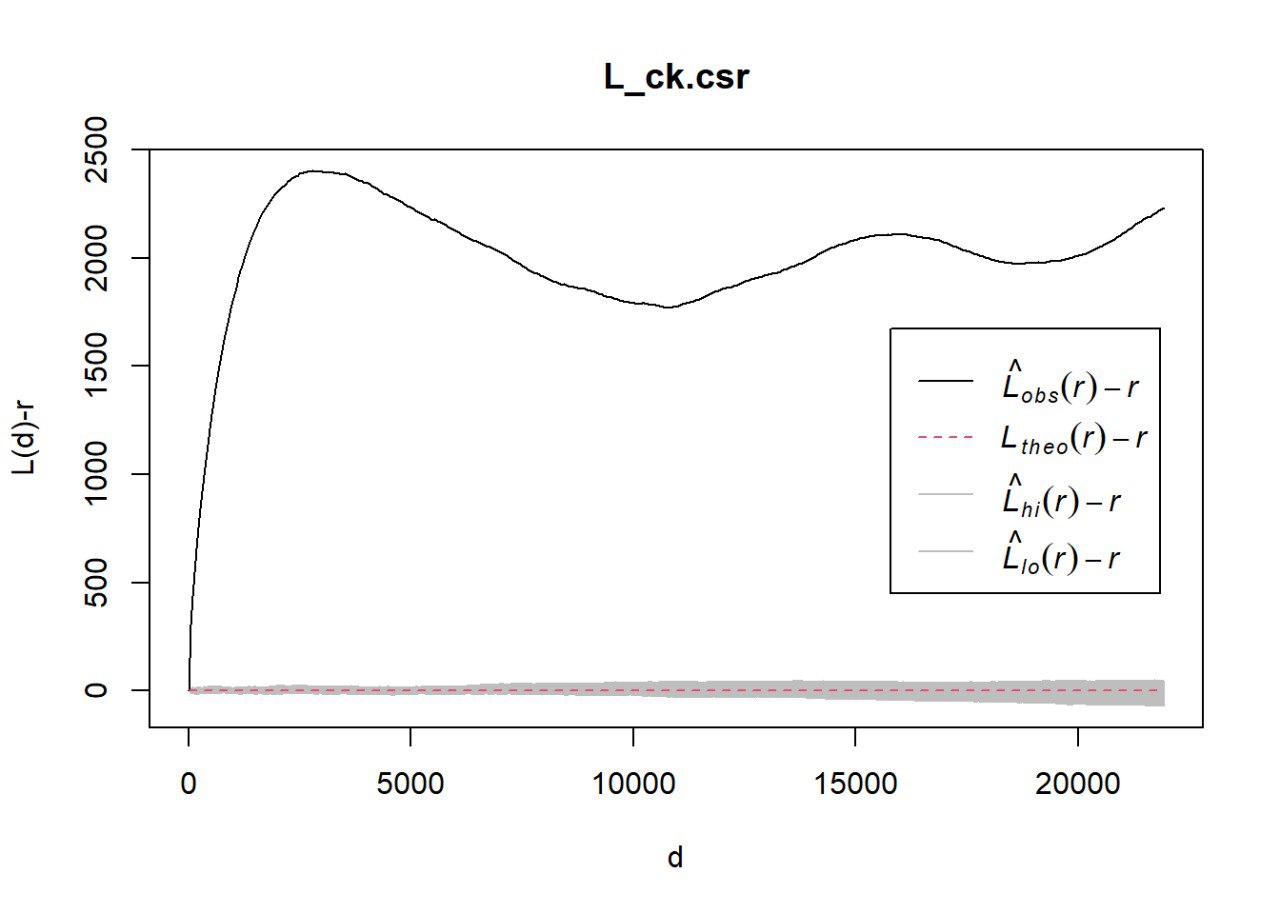
As shown in the chart, given the L_ck.csr plotted graph exited the envelope this shows that it is lesser than 0.05 of 95% confidence interval, H0 is rejected and we can conclude that the distribution of waterpoints are not randomly distributed.
11 Local Colocation Quotients (LCLQ)
Note:
The following code chunks above are commented to allow the take_home_ex1.html file (over 70mb) to commit and push to my github repository. The images from section 11 onwards are statically pasted to reduce the file size.
Before we perform the local colocation quotients, We will the wpdx_sf_nga dataframes to include both functional and non-functional water points only.
wpdx_lclq <- wpdx_sf_nga %>%
filter(status_clean %in%
c("Functional",
"Non-Functional"))11.1 Visualizing the sf layer
Firstly, we want to visualise and observe how the sf layer will look like with the water points in osun.
#tmap_mode("view")
#tm_shape(osun) +
#tm_polygons() +
#tm_shape(wpdx_lclq) +
#tm_dots(col = "status_clean",
#size = 0.01,
#border.col = "black",
#border.lwd = 0.5)11.2 Applying Local Colocation Quotients (LCLQ)
In this section, we will perform the Local Colocation Quotients (LCLQ) to measure the concentration of the waterpoints in Osun by using local_colocation.
After visualising the sf layers, it looks like most waterpoints in the Osun state are highly concentrated. Thus, the test hypotheses are:
Ho = The concentration of the waterpoints in the Osun generally low
H1= The concentration of the waterpoints in the Osun state are generally high
To perform the Local Colocation Quotients (LCLQ), we will first identify the k nearest neighbors for given point geometry.
#nb <- include_self(
#st_knn(st_geometry(wpdx_lclq), 6))After that, we will create a weights list using a kernel function.
#wt <- st_kernel_weights(nb,
#wpdx_lclq,
#"gaussian",
#adaptive = TRUE)We will filter functional and non-functional from the wpdx_lclq whereby Functional will be A and Nonfunctional will be B.
#Functional <- wpdx_lclq %>%
#(status_clean == "Functional")
#A <- Functional$status_clean#NonFunctional <- wpdx_lclq %>%
#(status_clean == "Non-Functional")
#B <- NonFunctional$status_cleanWe will use the local_colocation() to calculate LCLQ.
#LCLQ <- local_colocation(A, B, nb, wt , 20)After that, we will use the column bind function to merge two data frames together given that the number of rows in both the data frames are equal.
#LCLQ_sf_nga <- cbind(wpdx_lclq, LCLQ)Finally, we will use the tmap() to visualise the results of LCLQ.
#tmap_mode("view")
#tm_shape(osun) +
#tm_polygons() +
#tm_shape(LCLQ_sf_nga) +
#tm_dots(col = "Non.Functional",
#size = 0.01,
#border.col = "black",
#border.lwd = 0.5)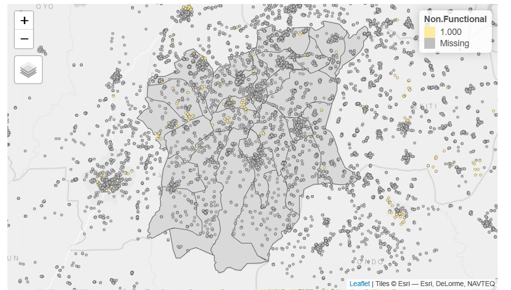
From the visualisation above, we can conclude that there are many ‘missing’ water points in Osun which implies that the points on the upper side of Osun State are more concentrated. Thus, we will reject H1 for this case since the concentration are generally low.
After performing the ‘clark evans test’, ‘L function’ and the ‘local colocation quotients’, we can conclude that H0 is rejected, the functional and non functional water points in Osun State are not randomly distributed with low concentration where the upper part of Osun state are slightly more concentrated.
End of take home exercise 1