Take Home Exercise 2

Author

Harith Oh Yee Choon

Published

February 20, 2023

Modified

March 2, 2023

Take-home Exercise 2: Spatio-temporal Analysis of COVID-19 Vaccination Trends at the Sub-district Level, DKI Jakarta

Setting the Scene

Since late December 2019, an outbreak of a novel coronavirus disease (COVID-19; previously known as 2019-nCoV) was reported in Wuhan, China, which had subsequently affected 210 countries worldwide. In general, COVID-19 is an acute resolved disease but it can also be deadly, with a 2% case fatality rate.

The COVID-19 vaccination in Indonesia is an ongoing mass immunisation in response to the COVID-19 pandemic in Indonesia. On 13 January 2021, the program commenced when President Joko Widodo was vaccinated at the presidential palace. In terms of total doses given, Indonesia ranks third in Asia and fifth in the world.

According to wikipedia, as of 5 February 2023 at 18:00 WIB (UTC+7), 204,266,655 people had received the first dose of the vaccine and 175,131,893 people had been fully vaccinated; 69,597,474 of them had been inoculated with the booster or the third dose, while 1,585,164 had received the fourth dose. Jakarta has the highest percentage of population fully vaccinated with 103.46%, followed by Bali and Special Region of Yogyakarta with 85.45% and 83.02% respectively.

Despite its compactness, the cumulative vaccination rate are not evenly distributed within DKI Jakarta. The question is where are the sub-districts with relatively higher number of vaccination rate and how they changed over time.

Objectives

Exploratory Spatial Data Analysis (ESDA) hold tremendous potential to address complex problems facing society. In this study, you are tasked to apply appropriate Local Indicators of Spatial Association (LISA) and Emerging Hot Spot Analysis (EHSA) to undercover the spatio-temporal trends of COVID-19 vaccination in DKI Jakarta.

f## The Task

The specific tasks of this take-home exercise are as follows:

Choropleth Mapping and Analysis

Compute the monthly vaccination rate from July 2021 to June 2022 at sub-district (also known as kelurahan in Bahasa Indonesia) level,
Prepare the monthly vaccination rate maps by using appropriate tmap functions,
Describe the spatial patterns revealed by the choropleth maps (not more than 200 words).

Local Gi* Analysis

With reference to the vaccination rate maps prepared in ESDA:

Compute local Gi* values of the monthly vaccination rate,
Display the Gi* maps of the monthly vaccination rate. The maps should only display the significant (i.e. p-value < 0.05)
With reference to the analysis results, draw statistical conclusions (not more than 250 words).

Emerging Hot Spot Analysis (EHSA)

With reference to the local Gi* values of the vaccination rate maps prepared in the previous section:

Perform Mann-Kendall Test by using the spatio-temporal local Gi* values,
Select three sub-districts and describe the temporal trends revealed (not more than 250 words), and
Prepared a EHSA map of the Gi* values of vaccination rate. The maps should only display the significant (i.e. p-value < 0.05).
With reference to the EHSA map prepared, describe the spatial patterns revealed. (not more than 250 words).

The Data

Aspatial data

For the purpose of this assignment, data from Riwayat File Vaksinasi DKI Jakarta will be used. Daily vaccination data are provides. You are only required to download either the first day of the month or last day of the month of the study period.

Geospatial data

For the purpose of this study, DKI Jakarta administration boundary 2019 will be used. The data set can be downloaded at Indonesia Geospatial portal, specifically at this page.

Note

The national Projected Coordinates Systems of Indonesia is DGN95 / Indonesia TM-3 zone 54.1.
Exclude all the outer islands from the DKI Jakarta sf data frame, and
Retain the first nine fields in the DKI Jakarta sf data frame. The ninth field JUMLAH_PEN = Total Population.
Reference was taken from the senior sample submissions for the code for this section, with credit to Megan - https://is415-msty.netlify.app/posts/2021-09-10-take-home-exercise-1/

1. Installing and Loading R packages

In this take home exercise 2, 9 packages will used and loaded using pacman.

pacman::p_load(sf, tmap, kableExtra, tidyverse, sfdep, readxl, plyr, Kendall, plotly)

1.1 Importing the Geospatial Data

The code chunk below uses st_read() of sf package to import BATAS_DESA_DESEMBER_2019_DUKCAPIL_DKI_JAKARTA shapefile into R. The imported shapefile will be simple features Object of sf. As we can see, the assigned coordinates system is WGS 84, the ‘World Geodetic System 1984’. In the context of this dataset, this isn’t appropriate: as this is an Indonesian-specific geospatial dataset, we should be using the national CRS of Indonesia, DGN95, the ‘Datum Geodesi Nasional 1995’, ESPG code 23845. st_transform will be used to rectify the coordinate system

bd_jakarta <- st_read(dsn = "data/Geospatial", 
                 layer = "BATAS_DESA_DESEMBER_2019_DUKCAPIL_DKI_JAKARTA")

Reading layer `BATAS_DESA_DESEMBER_2019_DUKCAPIL_DKI_JAKARTA' from data source 
  `C:\Harith-oh\IS415-Harith\Take-home_Ex2\data\Geospatial' using driver `ESRI Shapefile'
Simple feature collection with 269 features and 161 fields
Geometry type: MULTIPOLYGON
Dimension:     XY
Bounding box:  xmin: 106.3831 ymin: -6.370815 xmax: 106.9728 ymax: -5.184322
Geodetic CRS:  WGS 84

From the output message we can see that there are 269 features and 161 fields. The assigned CRS is WGS 84, the ‘World Geodetic System 1984’. This is not right, and will be rectify that later.

1.2 Data Pre-Processing

1.2.1 Check for Missing Values

Now lets check if there are any missing values

bd_jakarta[rowSums(is.na(bd_jakarta))!=0,]

Simple feature collection with 2 features and 161 fields
Geometry type: MULTIPOLYGON
Dimension:     XY
Bounding box:  xmin: 106.8412 ymin: -6.154036 xmax: 106.8612 ymax: -6.144973
Geodetic CRS:  WGS 84
    OBJECT_ID KODE_DESA             DESA   KODE    PROVINSI KAB_KOTA KECAMATAN
243     25645  31888888     DANAU SUNTER 318888 DKI JAKARTA     <NA>      <NA>
244     25646  31888888 DANAU SUNTER DLL 318888 DKI JAKARTA     <NA>      <NA>
    DESA_KELUR JUMLAH_PEN JUMLAH_KK LUAS_WILAY KEPADATAN PERPINDAHA JUMLAH_MEN
243       <NA>          0         0          0         0          0          0
244       <NA>          0         0          0         0          0          0
    PERUBAHAN WAJIB_KTP SILAM KRISTEN KHATOLIK HINDU BUDHA KONGHUCU KEPERCAYAA
243         0         0     0       0        0     0     0        0          0
244         0         0     0       0        0     0     0        0          0
    PRIA WANITA BELUM_KAWI KAWIN CERAI_HIDU CERAI_MATI U0 U5 U10 U15 U20 U25
243    0      0          0     0          0          0  0  0   0   0   0   0
244    0      0          0     0          0          0  0  0   0   0   0   0
    U30 U35 U40 U45 U50 U55 U60 U65 U70 U75 TIDAK_BELU BELUM_TAMA TAMAT_SD SLTP
243   0   0   0   0   0   0   0   0   0   0          0          0        0    0
244   0   0   0   0   0   0   0   0   0   0          0          0        0    0
    SLTA DIPLOMA_I DIPLOMA_II DIPLOMA_IV STRATA_II STRATA_III BELUM_TIDA
243    0         0          0          0         0          0          0
244    0         0          0          0         0          0          0
    APARATUR_P TENAGA_PEN WIRASWASTA PERTANIAN NELAYAN AGAMA_DAN PELAJAR_MA
243          0          0          0         0       0         0          0
244          0          0          0         0       0         0          0
    TENAGA_KES PENSIUNAN LAINNYA GENERATED KODE_DES_1 BELUM_ MENGUR_ PELAJAR_
243          0         0       0      <NA>       <NA>      0       0        0
244          0         0       0      <NA>       <NA>      0       0        0
    PENSIUNA_1 PEGAWAI_ TENTARA KEPOLISIAN PERDAG_ PETANI PETERN_ NELAYAN_1
243          0        0       0          0       0      0       0         0
244          0        0       0          0       0      0       0         0
    INDUSTR_ KONSTR_ TRANSP_ KARYAW_ KARYAW1 KARYAW1_1 KARYAW1_12 BURUH BURUH_
243        0       0       0       0       0         0          0     0      0
244        0       0       0       0       0         0          0     0      0
    BURUH1 BURUH1_1 PEMBANT_ TUKANG TUKANG_1 TUKANG_12 TUKANG__13 TUKANG__14
243      0        0        0      0        0         0          0          0
244      0        0        0      0        0         0          0          0
    TUKANG__15 TUKANG__16 TUKANG__17 PENATA PENATA_ PENATA1_1 MEKANIK SENIMAN_
243          0          0          0      0       0         0       0        0
244          0          0          0      0       0         0       0        0
    TABIB PARAJI_ PERANCA_ PENTER_ IMAM_M PENDETA PASTOR WARTAWAN USTADZ JURU_M
243     0       0        0       0      0       0      0        0      0      0
244     0       0        0       0      0       0      0        0      0      0
    PROMOT ANGGOTA_ ANGGOTA1 ANGGOTA1_1 PRESIDEN WAKIL_PRES ANGGOTA1_2
243      0        0        0          0        0          0          0
244      0        0        0          0        0          0          0
    ANGGOTA1_3 DUTA_B GUBERNUR WAKIL_GUBE BUPATI WAKIL_BUPA WALIKOTA WAKIL_WALI
243          0      0        0          0      0          0        0          0
244          0      0        0          0      0          0        0          0
    ANGGOTA1_4 ANGGOTA1_5 DOSEN GURU PILOT PENGACARA_ NOTARIS ARSITEK AKUNTA_
243          0          0     0    0     0          0       0       0       0
244          0          0     0    0     0          0       0       0       0
    KONSUL_ DOKTER BIDAN PERAWAT APOTEK_ PSIKIATER PENYIA_ PENYIA1 PELAUT
243       0      0     0       0       0         0       0       0      0
244       0      0     0       0       0         0       0       0      0
    PENELITI SOPIR PIALAN PARANORMAL PEDAGA_ PERANG_ KEPALA_ BIARAW_ WIRASWAST_
243        0     0      0          0       0       0       0       0          0
244        0     0      0          0       0       0       0       0          0
    LAINNYA_12 LUAS_DESA KODE_DES_3 DESA_KEL_1 KODE_12
243          0         0       <NA>       <NA>       0
244          0         0       <NA>       <NA>       0
                          geometry
243 MULTIPOLYGON (((106.8612 -6...
244 MULTIPOLYGON (((106.8504 -6...

There are 2 rows containing ‘NA’ values. However, the data is big, we need to find columns with missing NA values to remove it.

names(which(colSums(is.na(bd_jakarta))>0))

[1] "KAB_KOTA"   "KECAMATAN"  "DESA_KELUR" "GENERATED"  "KODE_DES_1"
[6] "KODE_DES_3" "DESA_KEL_1"

We can see that there are two particular rows with missing values for KAB_KOTA (City), KECAMATAN (District) and DESA_KELUR (Village).

Hence, we remove rows with NA value in DESA_KELUR. There are other columns with NA present as well, however, since we are only looking at the sub-district level, it is most appropriate to remove DESA_KELUR.

bd_jakarta <- na.omit(bd_jakarta,c("DESA_KELUR"))

To double check if the rows with missing values are removed

bd_jakarta[rowSums(is.na(bd_jakarta))!=0,]

Simple feature collection with 0 features and 161 fields
Bounding box:  xmin: NA ymin: NA xmax: NA ymax: NA
Geodetic CRS:  WGS 84
  [1] OBJECT_ID  KODE_DESA  DESA       KODE       PROVINSI   KAB_KOTA  
  [7] KECAMATAN  DESA_KELUR JUMLAH_PEN JUMLAH_KK  LUAS_WILAY KEPADATAN 
 [13] PERPINDAHA JUMLAH_MEN PERUBAHAN  WAJIB_KTP  SILAM      KRISTEN   
 [19] KHATOLIK   HINDU      BUDHA      KONGHUCU   KEPERCAYAA PRIA      
 [25] WANITA     BELUM_KAWI KAWIN      CERAI_HIDU CERAI_MATI U0        
 [31] U5         U10        U15        U20        U25        U30       
 [37] U35        U40        U45        U50        U55        U60       
 [43] U65        U70        U75        TIDAK_BELU BELUM_TAMA TAMAT_SD  
 [49] SLTP       SLTA       DIPLOMA_I  DIPLOMA_II DIPLOMA_IV STRATA_II 
 [55] STRATA_III BELUM_TIDA APARATUR_P TENAGA_PEN WIRASWASTA PERTANIAN 
 [61] NELAYAN    AGAMA_DAN  PELAJAR_MA TENAGA_KES PENSIUNAN  LAINNYA   
 [67] GENERATED  KODE_DES_1 BELUM_     MENGUR_    PELAJAR_   PENSIUNA_1
 [73] PEGAWAI_   TENTARA    KEPOLISIAN PERDAG_    PETANI     PETERN_   
 [79] NELAYAN_1  INDUSTR_   KONSTR_    TRANSP_    KARYAW_    KARYAW1   
 [85] KARYAW1_1  KARYAW1_12 BURUH      BURUH_     BURUH1     BURUH1_1  
 [91] PEMBANT_   TUKANG     TUKANG_1   TUKANG_12  TUKANG__13 TUKANG__14
 [97] TUKANG__15 TUKANG__16 TUKANG__17 PENATA     PENATA_    PENATA1_1 
[103] MEKANIK    SENIMAN_   TABIB      PARAJI_    PERANCA_   PENTER_   
[109] IMAM_M     PENDETA    PASTOR     WARTAWAN   USTADZ     JURU_M    
[115] PROMOT     ANGGOTA_   ANGGOTA1   ANGGOTA1_1 PRESIDEN   WAKIL_PRES
[121] ANGGOTA1_2 ANGGOTA1_3 DUTA_B     GUBERNUR   WAKIL_GUBE BUPATI    
[127] WAKIL_BUPA WALIKOTA   WAKIL_WALI ANGGOTA1_4 ANGGOTA1_5 DOSEN     
[133] GURU       PILOT      PENGACARA_ NOTARIS    ARSITEK    AKUNTA_   
[139] KONSUL_    DOKTER     BIDAN      PERAWAT    APOTEK_    PSIKIATER 
[145] PENYIA_    PENYIA1    PELAUT     PENELITI   SOPIR      PIALAN    
[151] PARANORMAL PEDAGA_    PERANG_    KEPALA_    BIARAW_    WIRASWAST_
[157] LAINNYA_12 LUAS_DESA  KODE_DES_3 DESA_KEL_1 KODE_12    geometry  
<0 rows> (or 0-length row.names)

1.2.2 Transforming Coordinates

Previously as mentioned it uses the WGS 84 coordinate system. The data is using a Geographic projected system, however, this is system is not appropriate since we need to use distance and area measures.

st_crs(bd_jakarta)

Coordinate Reference System:
  User input: WGS 84 
  wkt:
GEOGCRS["WGS 84",
    DATUM["World Geodetic System 1984",
        ELLIPSOID["WGS 84",6378137,298.257223563,
            LENGTHUNIT["metre",1]]],
    PRIMEM["Greenwich",0,
        ANGLEUNIT["degree",0.0174532925199433]],
    CS[ellipsoidal,2],
        AXIS["latitude",north,
            ORDER[1],
            ANGLEUNIT["degree",0.0174532925199433]],
        AXIS["longitude",east,
            ORDER[2],
            ANGLEUNIT["degree",0.0174532925199433]],
    ID["EPSG",4326]]

Therefore, we use st_transform() and not st_set_crs() as st_set_crs() assigns the EPSG code to the data frame. And we need to transform the data frame from geographic to projected coordinate system. We will be using crs=23845 (found from the EPSG for Indonesia).

bd_jakarta <- st_transform(bd_jakarta, 23845)

Check if CRS has been assigned

st_crs(bd_jakarta)

Coordinate Reference System:
  User input: EPSG:23845 
  wkt:
PROJCRS["DGN95 / Indonesia TM-3 zone 54.1",
    BASEGEOGCRS["DGN95",
        DATUM["Datum Geodesi Nasional 1995",
            ELLIPSOID["WGS 84",6378137,298.257223563,
                LENGTHUNIT["metre",1]]],
        PRIMEM["Greenwich",0,
            ANGLEUNIT["degree",0.0174532925199433]],
        ID["EPSG",4755]],
    CONVERSION["Indonesia TM-3 zone 54.1",
        METHOD["Transverse Mercator",
            ID["EPSG",9807]],
        PARAMETER["Latitude of natural origin",0,
            ANGLEUNIT["degree",0.0174532925199433],
            ID["EPSG",8801]],
        PARAMETER["Longitude of natural origin",139.5,
            ANGLEUNIT["degree",0.0174532925199433],
            ID["EPSG",8802]],
        PARAMETER["Scale factor at natural origin",0.9999,
            SCALEUNIT["unity",1],
            ID["EPSG",8805]],
        PARAMETER["False easting",200000,
            LENGTHUNIT["metre",1],
            ID["EPSG",8806]],
        PARAMETER["False northing",1500000,
            LENGTHUNIT["metre",1],
            ID["EPSG",8807]]],
    CS[Cartesian,2],
        AXIS["easting (X)",east,
            ORDER[1],
            LENGTHUNIT["metre",1]],
        AXIS["northing (Y)",north,
            ORDER[2],
            LENGTHUNIT["metre",1]],
    USAGE[
        SCOPE["Cadastre."],
        AREA["Indonesia - onshore east of 138°E."],
        BBOX[-9.19,138,-1.49,141.01]],
    ID["EPSG",23845]]

1.2.3 Removal of the Outer Island

We have done our basic pre-processing, lets quickly visualize the data

plot(st_geometry(bd_jakarta))

As we can see from the diagram, bd_jakarta includes both mainland and outer islands. And since we don’t require the outer islands (as per the requirements), we can remove them.

We know that the date is grouped by KAB_KOTA (City), KECAMATAN (Sub-District) and DESA_KELUR (Village). Now, lets plot the map and see how we can use KAB_KOTA to remove the outer islands.

tm_shape(bd_jakarta) + 
  tm_polygons("KAB_KOTA")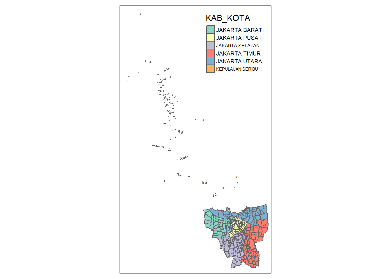

From the map, we can see that all the cities in Jakarta start with ‘Jakarta’ as their prefix and hence, ‘Kepulauan Seribu’ are the other outer islands. When translated in English, the name means ‘Thousand Islands’. Now we know what to remove, and we shall proceed with that.

bd_jakarta <- filter(bd_jakarta, KAB_KOTA != "KEPULAUAN SERIBU")

Now, lets double check if the outer islands have been removed.

tm_shape(bd_jakarta) + 
  tm_polygons("KAB_KOTA")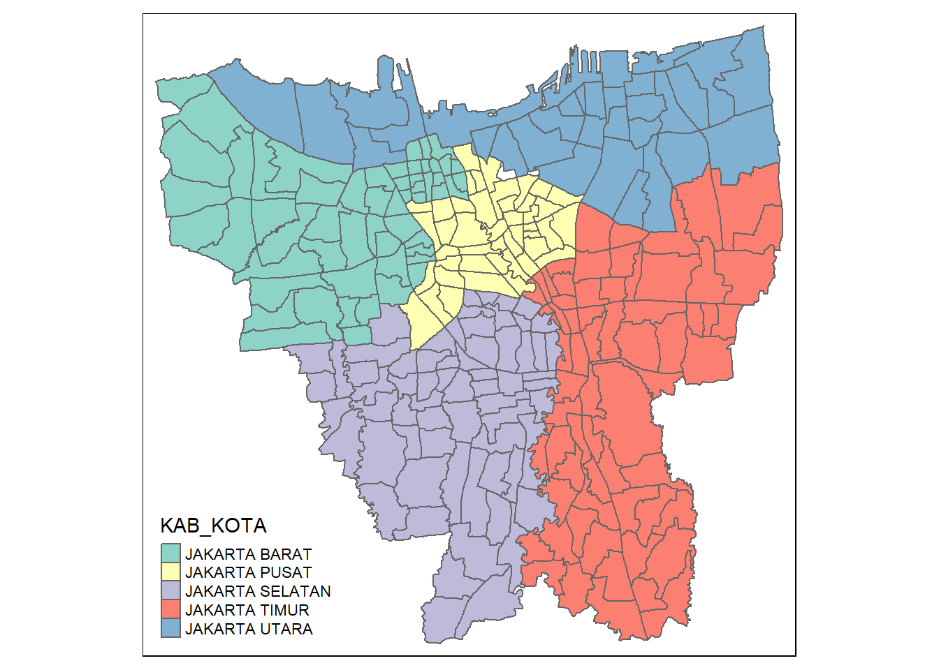

1.2.4 To retain the first 9 columns as requested

bd_jakarta <- bd_jakarta[, 0:9]

1.2.5 Renaming columns to English

bd_jakarta <- bd_jakarta %>% 
  dplyr::rename(
    Object_ID=OBJECT_ID,
    Village_Code=KODE_DESA, 
    Village=DESA,
    Code=KODE,
    Province=PROVINSI, 
    City=KAB_KOTA, 
    District=KECAMATAN, 
    Sub_District=DESA_KELUR,
    Total_Population=JUMLAH_PEN
    )

2. Data Wrangling for Aspatial Data

2.1 Importing EDA

For this take home exercise 2, we will be working on data from July 2021 to June 2022, as a result we will be having several excel files.

jul2021 <- read_xlsx("data/Aspatial/Data Vaksinasi Berbasis Kelurahan (31 Juli 2021).xlsx")

glimpse(jul2021)

Rows: 268
Columns: 27
$ `KODE KELURAHAN`                             <chr> NA, "3172051003", "317304…
$ `WILAYAH KOTA`                               <chr> NA, "JAKARTA UTARA", "JAK…
$ KECAMATAN                                    <chr> NA, "PADEMANGAN", "TAMBOR…
$ KELURAHAN                                    <chr> "TOTAL", "ANCOL", "ANGKE"…
$ SASARAN                                      <dbl> 8941211, 23947, 29381, 29…
$ `BELUM VAKSIN`                               <dbl> 4441501, 12333, 13875, 18…
$ `JUMLAH\r\nDOSIS 1`                          <dbl> 4499710, 11614, 15506, 10…
$ `JUMLAH\r\nDOSIS 2`                          <dbl> 1663218, 4181, 4798, 3658…
$ `TOTAL VAKSIN\r\nDIBERIKAN`                  <dbl> 6162928, 15795, 20304, 14…
$ `LANSIA\r\nDOSIS 1`                          <dbl> 502579, 1230, 2012, 865, …
$ `LANSIA\r\nDOSIS 2`                          <dbl> 440910, 1069, 1729, 701, …
$ `LANSIA TOTAL \r\nVAKSIN DIBERIKAN`          <dbl> 943489, 2299, 3741, 1566,…
$ `PELAYAN PUBLIK\r\nDOSIS 1`                  <dbl> 1052883, 3333, 2586, 2837…
$ `PELAYAN PUBLIK\r\nDOSIS 2`                  <dbl> 666009, 2158, 1374, 1761,…
$ `PELAYAN PUBLIK TOTAL\r\nVAKSIN DIBERIKAN`   <dbl> 1718892, 5491, 3960, 4598…
$ `GOTONG ROYONG\r\nDOSIS 1`                   <dbl> 56660, 78, 122, 174, 71, …
$ `GOTONG ROYONG\r\nDOSIS 2`                   <dbl> 38496, 51, 84, 106, 57, 7…
$ `GOTONG ROYONG TOTAL\r\nVAKSIN DIBERIKAN`    <dbl> 95156, 129, 206, 280, 128…
$ `TENAGA KESEHATAN\r\nDOSIS 1`                <dbl> 76397, 101, 90, 215, 73, …
$ `TENAGA KESEHATAN\r\nDOSIS 2`                <dbl> 67484, 91, 82, 192, 67, 3…
$ `TENAGA KESEHATAN TOTAL\r\nVAKSIN DIBERIKAN` <dbl> 143881, 192, 172, 407, 14…
$ `TAHAPAN 3\r\nDOSIS 1`                       <dbl> 2279398, 5506, 9012, 5408…
$ `TAHAPAN 3\r\nDOSIS 2`                       <dbl> 446028, 789, 1519, 897, 4…
$ `TAHAPAN 3 TOTAL\r\nVAKSIN DIBERIKAN`        <dbl> 2725426, 6295, 10531, 630…
$ `REMAJA\r\nDOSIS 1`                          <dbl> 531793, 1366, 1684, 1261,…
$ `REMAJA\r\nDOSIS 2`                          <dbl> 4291, 23, 10, 1, 1, 8, 6,…
$ `REMAJA TOTAL\r\nVAKSIN DIBERIKAN`           <dbl> 536084, 1389, 1694, 1262,…

From opening up the excel file till February 2022, the number of columns is 27. However, from March 2022 the number of columns is 34. Upon identifying the difference between the number of columns, the data files from March 2022 has a separate column for 3rd dosage, where has all the data files before that don’t have 3rd dosage column.

2.2 Creating Aspatial Data Pre-Processing Function

For take home exercise 2, we don’t require all the columns. Only the following columns are required -

KODE KELURAHAN (Sub-District Code)

KELURAHAN (Sub-District)

SASARAN (Target)

BELUM VASKIN (Yet to be vaccinated / Not yet vaccinated)

This solves the issue of some months having extra columns. However, we need to create an ‘Date’ column that shows the month and year of the observation, which is originally the file name. Each file has the naming convention ’Data Vaksinasi Berbasis Keluarahan (DD Month YYYY).

We will be combining the mentioned steps into a function

# takes in an aspatial data filepath and returns a processed output
aspatial_preprocess <- function(filepath){
  # We have to remove the first row of the file (subheader row) and hence, we use [-1,] to remove it.
  result_file <- read_xlsx(filepath)[-1,]
  
  # We then create the Date Column, the format of our files is: Data Vaksinasi Berbasis Kelurahan (DD Month YYYY)
  # While the start is technically "(", "(" is part of a regular expression and leads to a warning message, so we'll use "Kelurahan" instead. The [[1]] refers to the first element in the list.
  # We're loading it as DD-Month-YYYY format
  # We use the length of the filepath '6' to get the end index (which has our Date)
  # as such, the most relevant functions are substr (returns a substring) and either str_locate (returns location of substring as an integer matrix) or gregexpr (returns a list of locations of substring)
  # reference https://stackoverflow.com/questions/14249562/find-the-location-of-a-character-in-string
  startpoint <- gregexpr(pattern="Kelurahan", filepath)[[1]] + 11
  
  result_file$Date <- substr(filepath, startpoint, nchar(filepath)-6)
  
  # Retain the Relevant Columns
  result_file <- result_file %>% 
    select("Date", 
           "KODE KELURAHAN", 
           "KELURAHAN", 
           "SASARAN", 
           "BELUM VAKSIN")
  return(result_file)
}

2.3 Feed files into Aspatial function

Instead of manually feeding the files, line by line, we will be using the function list.files() and lapply() to get our process done quicker.

# in the folder 'data/aspatial', find files with the extension '.xlsx' and add it to our fileslist 
# the full.names=TRUE prepends the directory path to the file names, giving a relative file path - otherwise, only the file names (not the paths) would be returned 
# reference: https://stat.ethz.ch/R-manual/R-devel/library/base/html/list.files.html
fileslist <-list.files(path = "data/Aspatial", pattern = "*.xlsx", full.names=TRUE)

# afterwards, for every element in fileslist, apply aspatial_process function
dflist <- lapply(seq_along(fileslist), function(x) aspatial_preprocess(fileslist[x]))

We will then convert the dflist into an actual dataframe with ldply() using the below code

vaccination_jakarta <- ldply(dflist, data.frame)

Now, lets take a look into our data

glimpse(vaccination_jakarta)

Rows: 3,204
Columns: 5
$ Date           <chr> "27 Februari 2022", "27 Februari 2022", "27 Februari 20…
$ KODE.KELURAHAN <chr> "3172051003", "3173041007", "3175041005", "3175031003",…
$ KELURAHAN      <chr> "ANCOL", "ANGKE", "BALE KAMBANG", "BALI MESTER", "BAMBU…
$ SASARAN        <dbl> 23947, 29381, 29074, 9752, 26285, 21566, 23886, 47898, …
$ BELUM.VAKSIN   <dbl> 4592, 5319, 5903, 1649, 4030, 3950, 3344, 9382, 3772, 7…

2.4 Formatting Date Column

The Dates are in Bahasa Indonesia, and hence, we need to translate them to English for ease of use. However, since the values in Date column were derived from sub-strings, they are in a string format and thus, first need to be converted to datetime.

# parses the 'Date' column into Month(Full Name)-YYYY datetime objects
# reference: https://stackoverflow.com/questions/53380650/b-y-date-conversion-gives-na

# locale="ind" means that the locale has been set as Indonesia
Sys.setlocale(locale="ind")

[1] "LC_COLLATE=Indonesian_Indonesia.1252;LC_CTYPE=Indonesian_Indonesia.1252;LC_MONETARY=Indonesian_Indonesia.1252;LC_NUMERIC=C;LC_TIME=Indonesian_Indonesia.1252"

vaccination_jakarta$Date <- c(vaccination_jakarta$Date) %>% 
  as.Date(vaccination_jakarta$Date, format ="%d %B %Y")

glimpse(vaccination_jakarta)

Rows: 3,204
Columns: 5
$ Date           <date> 2022-02-27, 2022-02-27, 2022-02-27, 2022-02-27, 2022-0~
$ KODE.KELURAHAN <chr> "3172051003", "3173041007", "3175041005", "3175031003",~
$ KELURAHAN      <chr> "ANCOL", "ANGKE", "BALE KAMBANG", "BALI MESTER", "BAMBU~
$ SASARAN        <dbl> 23947, 29381, 29074, 9752, 26285, 21566, 23886, 47898, ~
$ BELUM.VAKSIN   <dbl> 4592, 5319, 5903, 1649, 4030, 3950, 3344, 9382, 3772, 7~

2.5 Rename columns into English

# renames the columns in the style New_Name = OLD_NAME
vaccination_jakarta <- vaccination_jakarta %>% 
  dplyr::rename(
    Date=Date,
    Sub_District_Code=KODE.KELURAHAN,
    Sub_District=KELURAHAN, 
    Target=SASARAN, 
    Not_Yet_Vaccinated=BELUM.VAKSIN
    )

glimpse(vaccination_jakarta)

Rows: 3,204
Columns: 5
$ Date               <date> 2022-02-27, 2022-02-27, 2022-02-27, 2022-02-27, 20~
$ Sub_District_Code  <chr> "3172051003", "3173041007", "3175041005", "31750310~
$ Sub_District       <chr> "ANCOL", "ANGKE", "BALE KAMBANG", "BALI MESTER", "B~
$ Target             <dbl> 23947, 29381, 29074, 9752, 26285, 21566, 23886, 478~
$ Not_Yet_Vaccinated <dbl> 4592, 5319, 5903, 1649, 4030, 3950, 3344, 9382, 377~

2.6 Further data processing

Further perform any pre-processing to check out for anything we might have missed.

vaccination_jakarta[rowSums(is.na(vaccination_jakarta))!=0,]

[1] Date               Sub_District_Code  Sub_District       Target            
[5] Not_Yet_Vaccinated
<0 rows> (or 0-length row.names)

From the output, we can see there are no missing values.

3. Geospatial Data Integration

3.1 Initial Exploratory Data Analysis

We have both our Geospatial and Aspatial data, we need to join them. However, we need to first find a common header to join them.

colnames(bd_jakarta)

 [1] "Object_ID"        "Village_Code"     "Village"          "Code"            
 [5] "Province"         "City"             "District"         "Sub_District"    
 [9] "Total_Population" "geometry"

colnames(vaccination_jakarta)

[1] "Date"               "Sub_District_Code"  "Sub_District"      
[4] "Target"             "Not_Yet_Vaccinated"

We can see that both have Sub_District and hence we can join them by the Sub_District and Sub_District_Code.

# joins vaccination_jakarta to jakarta based on Sub_District and  Sub_District_Code
combined_jakarta <- left_join(bd_jakarta, vaccination_jakarta,
                              by=c(
                                "Village_Code"="Sub_District_Code", 
                                "Sub_District"="Sub_District")
                              )

Subcategorize the data into ‘Target population to be Vaccinated’ , ‘Not Yet Vaccinated Population’ and ‘Total Population’

target = tm_shape(combined_jakarta)+
  tm_fill("Target") +
  tm_borders(alpha = 0.5) +
  tm_layout(main.title="Target Count")

not_yet_vaccinated = tm_shape(combined_jakarta)+
  tm_fill("Not_Yet_Vaccinated") +
  tm_borders(alpha = 0.5) +
  tm_layout(main.title="Not Yet Vaccinated Count")

total_population = tm_shape(combined_jakarta)+
  tm_fill("Total_Population") +
  tm_borders(alpha = 0.5) +
  tm_layout(main.title="Total Population")

tmap_arrange(target, not_yet_vaccinated, total_population)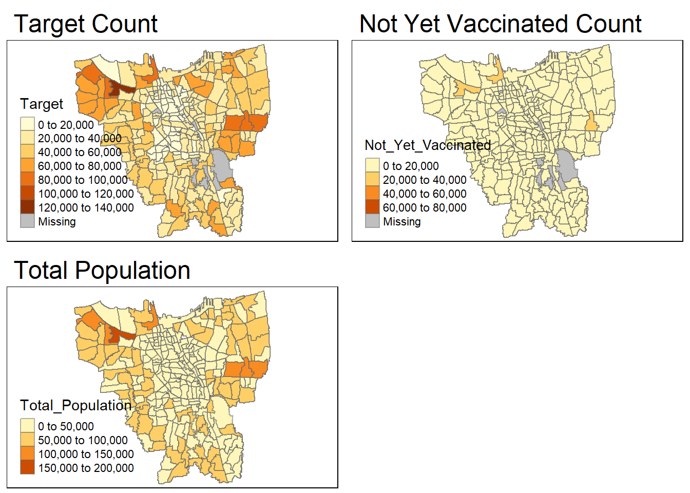

There seems to be still be a ‘Missing’ value in the Target and Not_Yet_Vaccinated maps. Even though, when we had previously checked for missing values, it didn’t show any missing values. However, we shall double check again.

bd_jakarta[rowSums(is.na(bd_jakarta))!=0,]

Simple feature collection with 0 features and 9 fields
Bounding box:  xmin: NA ymin: NA xmax: NA ymax: NA
Projected CRS: DGN95 / Indonesia TM-3 zone 54.1
 [1] Object_ID        Village_Code     Village          Code            
 [5] Province         City             District         Sub_District    
 [9] Total_Population geometry        
<0 rows> (or 0-length row.names)

vaccination_jakarta[rowSums(is.na(vaccination_jakarta))!=0,]

[1] Date               Sub_District_Code  Sub_District       Target            
[5] Not_Yet_Vaccinated
<0 rows> (or 0-length row.names)

There are no missing values in our dataframes. Therefore, the most likely reasons for the missing values must be due to mismatched values when we perform the left-join of the Geospatial and Aspatial data.

3.2 Finding mismatched sub-district records

Since, we had conducted left-join using the Sub-District, there must be a mismatch in the naming of the subdistricts. Lets check it by looking at the unique subdistrict names in both bd_jakarta and vaccination_jakarta

jakarta_subdistrict <- c(bd_jakarta$Sub_District)
vaccination_subdistrict <- c(vaccination_jakarta$Sub_District)

unique(jakarta_subdistrict[!(jakarta_subdistrict %in% vaccination_subdistrict)])

[1] "KRENDANG"             "RAWAJATI"             "TENGAH"              
[4] "BALEKAMBANG"          "PINANGRANTI"          "JATIPULO"            
[7] "PALMERIAM"            "KRAMATJATI"           "HALIM PERDANA KUSUMA"

unique(vaccination_subdistrict[!(vaccination_subdistrict %in% jakarta_subdistrict)])

 [1] "BALE KAMBANG"          "HALIM PERDANA KUSUMAH" "JATI PULO"            
 [4] "KAMPUNG TENGAH"        "KERENDANG"             "KRAMAT JATI"          
 [7] "PAL MERIAM"            "PINANG RANTI"          "PULAU HARAPAN"        
[10] "PULAU KELAPA"          "PULAU PANGGANG"        "PULAU PARI"           
[13] "PULAU TIDUNG"          "PULAU UNTUNG JAWA"     "RAWA JATI"

From above there are same names in both but are just written in different ways. However, there are 6 words in the vaccination_subdistrict which are not in the jakarta_subdistrict. We need to take a look into that after we first correct the mismatched values.

# initialise a dataframe of our cases vs bd subdistrict spelling
spelling <- data.frame(
  Aspatial_Cases=c("BALE KAMBANG", "HALIM PERDANA KUSUMAH", "JATI PULO", "KAMPUNG TENGAH", "KERENDANG", "KRAMAT JATI", "PAL MERIAM", "PINANG RANTI", "RAWA JATI"),
  Geospatial_BD=c("BALEKAMBAG", "HALIM PERDANA KUSUMA", "JATIPULO", "TENGAH", "KRENDANG", "KRAMATJATI", "PALMERIAM", "PINANGRANTI", "RAWAJATI")
  )

# with dataframe a input, outputs a kable
library(knitr)
library(kableExtra)
kable(spelling, caption="Mismatched Records") %>%
  kable_material("hover", latex_options="scale_down")

Mismatched Records
Aspatial_Cases	Geospatial_BD
BALE KAMBANG	BALEKAMBAG
HALIM PERDANA KUSUMAH	HALIM PERDANA KUSUMA
JATI PULO	JATIPULO
KAMPUNG TENGAH	TENGAH
KERENDANG	KRENDANG
KRAMAT JATI	KRAMATJATI
PAL MERIAM	PALMERIAM
PINANG RANTI	PINANGRANTI
RAWA JATI	RAWAJATI

As we can see these records have the same name, except that there is no standardization. Therefore, there is a mismatch between them. Let’s correct this mismatch

# We are replacing the mistmatched values in jakarta with the correct value
bd_jakarta$Sub_District[bd_jakarta$Sub_District == 'BALEKAMBANG'] <- 'BALE KAMBANG'
bd_jakarta$Sub_District[bd_jakarta$Sub_District == 'HALIM PERDANA KUSUMA'] <- 'HALIM PERDANA KUSUMAH'
bd_jakarta$Sub_District[bd_jakarta$Sub_District == 'JATIPULO'] <- 'JATI PULO'
bd_jakarta$Sub_District[bd_jakarta$Sub_District == 'KALI BARU'] <- 'KALIBARU'
bd_jakarta$Sub_District[bd_jakarta$Sub_District == 'TENGAH'] <- 'KAMPUNG TENGAH'
bd_jakarta$Sub_District[bd_jakarta$Sub_District == 'KRAMATJATI'] <- 'KRAMAT JATI'
bd_jakarta$Sub_District[bd_jakarta$Sub_District == 'KRENDANG'] <- 'KERENDANG'
bd_jakarta$Sub_District[bd_jakarta$Sub_District == 'PALMERIAM'] <- 'PAL MERIAM'
bd_jakarta$Sub_District[bd_jakarta$Sub_District == 'PINANGRANTI'] <- 'PINANG RANTI'
bd_jakarta$Sub_District[bd_jakarta$Sub_District == 'RAWAJATI'] <- 'RAWA JATI'

There are 6 subdistrict names that we say in vaccination_jakarta which were not present in jakarta. This ideally suggests that these districts are not a part of Jakarta, Therefore we need to remove them.

vaccination_jakarta <- vaccination_jakarta[!(vaccination_jakarta$Sub_District=="PULAU HARAPAN" | vaccination_jakarta$Sub_District=="PULAU KELAPA" | vaccination_jakarta$Sub_District=="PULAU PANGGANG" | vaccination_jakarta$Sub_District=="PULAU PARI" | vaccination_jakarta$Sub_District=="PULAU TIDUNG" | vaccination_jakarta$Sub_District=="PULAU UNTUNG JAWA"), ]

3.3 Rejoin Exploratory Data Analysis

# joins vaccination_jakarta to bd_jakarta based on Sub_District and  Sub_District_Code
combined_jakarta <- left_join(bd_jakarta, vaccination_jakarta,
                              by=c(
                                "Village_Code"="Sub_District_Code", 
                                "Sub_District"="Sub_District")
                              )

Check if there are any further NA values

combined_jakarta[rowSums(is.na(combined_jakarta))!=0,]

Simple feature collection with 0 features and 12 fields
Bounding box:  xmin: NA ymin: NA xmax: NA ymax: NA
Projected CRS: DGN95 / Indonesia TM-3 zone 54.1
 [1] Object_ID          Village_Code       Village            Code              
 [5] Province           City               District           Sub_District      
 [9] Total_Population   Date               Target             Not_Yet_Vaccinated
[13] geometry          
<0 rows> (or 0-length row.names)

Relook the data into ‘Target population to be Vaccinated’ , ‘Not Yet Vaccinated Population’ and ‘Total Population’

target = tm_shape(combined_jakarta)+
  tm_fill("Target") +
  tm_borders(alpha = 0.5) +
  tm_layout(main.title="Target Count")

not_yet_vaccinated = tm_shape(combined_jakarta)+
  tm_fill("Not_Yet_Vaccinated") +
  tm_borders(alpha = 0.5) +
  tm_layout(main.title="Not Yet Vaccinated Count")

total_population = tm_shape(combined_jakarta)+
  tm_fill("Total_Population") +
  tm_borders(alpha = 0.5) +
  tm_layout(main.title="Total Population")

tmap_arrange(target, not_yet_vaccinated, total_population)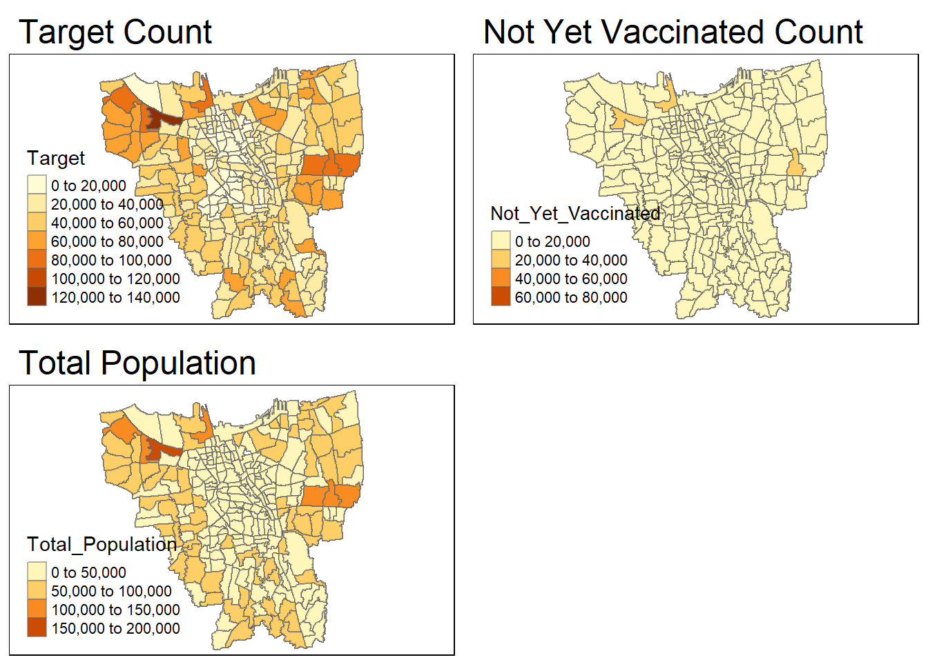

4. Calculation for monthly vaccination rate

We need to compute the monthly vaccination rate in % at the sub-district level.

We use ‘Target’ -SASARAN instead of Population because the government excludes people aged 14 and below for vaccination.

# grouping based on the sub-district and date
vaccination_rate <- vaccination_jakarta %>%
  inner_join(bd_jakarta, by=c("Sub_District" = "Sub_District")) %>%
  group_by(Sub_District, Date) %>%
  dplyr::summarise(`vaccination_rate` = ((Target-Not_Yet_Vaccinated)/Target)*100) %>%
  
  #afterwards, pivots the table based on the Dates, using the cumulative case rate as the values
  ungroup() %>% pivot_wider(names_from = Date,
              values_from = vaccination_rate)

Let us look into how the computation is

vaccination_rate

# A tibble: 261 x 13
   Sub_District  2021-~1 2021-~2 2021-~3 2021-~4 2021-~5 2021-~6 2022-~7 2022-~8
   <chr>           <dbl>   <dbl>   <dbl>   <dbl>   <dbl>   <dbl>   <dbl>   <dbl>
 1 ANCOL            48.5    61.6    72.1    75.0    76.9    78.9    80.6    80.8
 2 ANGKE            52.8    64.6    74.2    77.7    79.6    80.9    81.7    81.9
 3 BALE KAMBANG     37.0    57.0    70.0    73.9    76.6    78.2    79.5    79.7
 4 BALI MESTER      47.0    62.0    74.2    78.2    80.3    81.7    82.8    83.1
 5 BAMBU APUS       47.6    64.2    76.2    80.9    82.5    83.4    84.5    84.7
 6 BANGKA           51.6    61.3    73.2    78.0    79.8    80.7    81.5    81.7
 7 BARU             57.9    67.6    79.5    82.9    84.2    85.0    85.8    86.0
 8 BATU AMPAR       39.8    58.4    70.6    74.5    77.1    78.8    80.1    80.4
 9 BENDUNGAN HI~    53.6    62.6    75.6    79.1    80.5    81.4    82.3    82.5
10 BIDARA CINA      40.6    57.6    71.0    75.2    77.0    78.2    79.2    79.5
# ... with 251 more rows, 4 more variables: `2022-03-31` <dbl>,
#   `2022-04-30` <dbl>, `2022-05-31` <dbl>, `2022-06-30` <dbl>, and abbreviated
#   variable names 1: `2021-07-31`, 2: `2021-08-31`, 3: `2021-09-30`,
#   4: `2021-10-31`, 5: `2021-11-30`, 6: `2021-12-31`, 7: `2022-01-31`,
#   8: `2022-02-27`

4.1 Convert dataframe to SF

combined_jakarta <- st_as_sf(combined_jakarta)

# need to join our previous dataframes with the geospatial data to ensure that geometry column is present
vaccination_rate <- vaccination_rate%>% left_join(bd_jakarta, by=c("Sub_District"="Sub_District"))
vaccination_rate <- st_as_sf(vaccination_rate)

5 Choropleth Mapping and performing Analysis

There are a few ways to classify data in Choropleth maps such as using Equal Interval, Quantile or Jenks.

For this take home exercise 2, I will be using Jenks as this method uses statistical algorithm to group data into classes in the distribution of values. In addition it suits low variance. As a result it will accurately reflects the distribution of values in the data.

5.1 Jenks Choropleth Mapping

# using the jenks method, with 6 classes for human eye
tmap_mode("plot")
tm_shape(vaccination_rate)+
  tm_fill("2021-07-31", 
          n= 6,
          style = "jenks", 
          title = "Vaccination Rate") +
  tm_layout(main.title = "Vaccination Rate in July 2021",
            main.title.position = "center",
            main.title.size = 1,
            legend.height = 0.5, 
            legend.width = 0.4,
            frame = TRUE) +
  tm_borders(alpha = 0.5)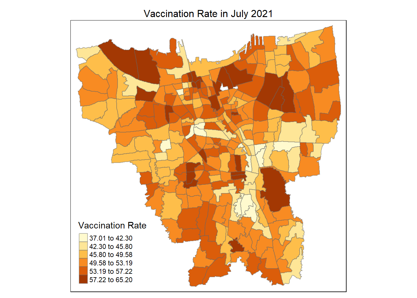

Plot for all 12 months. Adopt a helper function to help us do it.

# input: the dataframe and the variable name - in this case, the month 
# with style="jenks" for the jenks classification method
jenks_plot <- function(df, varname) {
  tm_shape(vaccination_rate) +
    tm_polygons() +
  tm_shape(df) +
    tm_fill(varname, 
          n= 6,
          style = "jenks", 
          title = "Vaccination Rate") +
    tm_layout(main.title = varname,
          main.title.position = "center",
          main.title.size = 1.2,
          legend.height = 0.45, 
          legend.width = 0.35,
          frame = TRUE) +
    tm_borders(alpha = 0.5)
}

tmap_mode("plot")
tmap_arrange(jenks_plot(vaccination_rate, "2021-07-31"),
             jenks_plot(vaccination_rate, "2021-08-31"),
             jenks_plot(vaccination_rate, "2021-09-30"),
             jenks_plot(vaccination_rate, "2021-10-31"))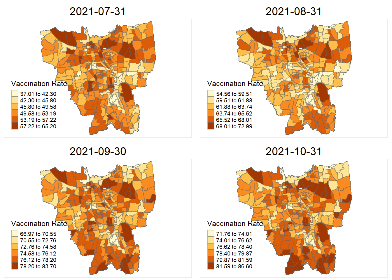

tmap_mode("plot")
tmap_arrange(jenks_plot(vaccination_rate, "2021-11-30"),
             jenks_plot(vaccination_rate, "2021-12-31"),
             jenks_plot(vaccination_rate, "2022-01-31"),
             jenks_plot(vaccination_rate, "2022-02-27"))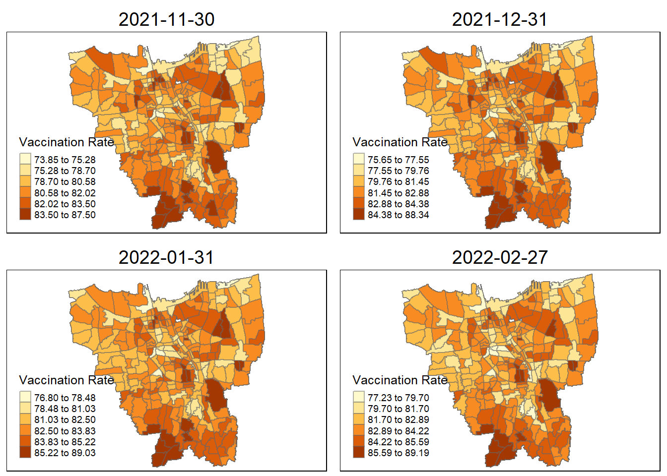

tmap_mode("plot")
tmap_arrange(jenks_plot(vaccination_rate, "2022-03-31"),
             jenks_plot(vaccination_rate, "2022-04-30"),
             jenks_plot(vaccination_rate, "2022-05-31"),
             jenks_plot(vaccination_rate, "2022-06-30"))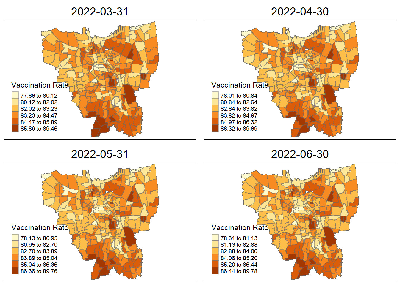

Observations from the plotted map

Each plotted map has been arranged monthly and has it own relative vaccination rate. As observed, the colours turns darker over time. As the ranges and gradually grow larger over time, more people are getting vaccinated.

By looking at the early stages between July 2021 and October 2021, there is a darkly-coloured cluster around the north of Jakarta which include KAMAL MUARA and HALIM PERDANA KUSUMAH sub-district with the highest vaccination rate.

As for other sub districts between (November 2021 ~ February 2022, other sub districts have darken in colour and the HALIM PERDANA KUSUMAH still remains the sub-district with the highest vaccination rate.

In the later stages of vaccination from March 2022, more sub-districts have lower vaccination rate (lighter colour) especially for the most of the sub-districts in the North and West. However, HALIM PERDANA KUSUMAH still remains the sub-district with the highest vaccination rate.

Checking for sub-districts with highest vaccination rate according to month

vaccination_rate$Sub_District[which.max(vaccination_rate$`2021-07-31`)]

[1] "KAMAL MUARA"

vaccination_rate$Sub_District[which.max(vaccination_rate$`2021-08-31`)]

[1] "KAMAL MUARA"

vaccination_rate$Sub_District[which.max(vaccination_rate$`2021-09-30`)]

[1] "HALIM PERDANA KUSUMAH"

vaccination_rate$Sub_District[which.max(vaccination_rate$`2021-10-31`)]

[1] "HALIM PERDANA KUSUMAH"

vaccination_rate$Sub_District[which.max(vaccination_rate$`2021-11-30`)]

[1] "HALIM PERDANA KUSUMAH"

vaccination_rate$Sub_District[which.max(vaccination_rate$`2021-12-31`)]

[1] "HALIM PERDANA KUSUMAH"

vaccination_rate$Sub_District[which.max(vaccination_rate$`2022-01-31`)]

[1] "HALIM PERDANA KUSUMAH"

vaccination_rate$Sub_District[which.max(vaccination_rate$`2022-02-27`)]

[1] "HALIM PERDANA KUSUMAH"

vaccination_rate$Sub_District[which.max(vaccination_rate$`2022-03-31`)]

[1] "HALIM PERDANA KUSUMAH"

vaccination_rate$Sub_District[which.max(vaccination_rate$`2022-04-30`)]

[1] "HALIM PERDANA KUSUMAH"

vaccination_rate$Sub_District[which.max(vaccination_rate$`2022-05-31`)]

[1] "HALIM PERDANA KUSUMAH"

vaccination_rate$Sub_District[which.max(vaccination_rate$`2022-06-31`)]

character(0)

6. Local GI* Analysis

A Local Gi* Analysis will be conducted. It is also known as local spatial autocorrelation which will be used to identify ideas sub-districts in Jakarta with high or low vaccination rate. Time-series analysis will be conducted to understand the evolution of spatial hot spots and cold spots across time.

Interpretation of Gi* values

Gi∗ > 0 which indicates sub-districts with higher vaccination rate than average

Gi∗ < 0 which indicates sub-districts with higher vaccination rate than average

6.1 Calculation of Local GI* of monthly vaccination rate

# Make new vaccination attribute table with Date, Sub_District, Target, Not_Yet_Vaccinated
vaccination_table <- combined_jakarta %>% select(10, 8, 11, 12) %>% st_drop_geometry()

# Adding a new field for Vaccination_Rate
vaccination_table$Vaccination_Rate <- ((vaccination_table$Target - vaccination_table$Not_Yet_Vaccinated) / vaccination_table$Target) *100

# Vaccination attribute table with just Date, Sub_District, Vaccination_Rate
vaccination_table <- tibble(vaccination_table %>% select(1,2,5))

6.2 Create Time Series Cube

vaccination_rate_st <- spacetime(vaccination_table, bd_jakarta,
                          .loc_col = "Sub_District",
                          .time_col = "Date")

Verify if vaccination_rate_st is indeed a space-time cube by using the is_spacetime_cube() of sfdep package.

is_spacetime_cube(vaccination_rate_st)

[1] TRUE

6.3 Deriving Spatial Weights

Calculation of local Gi* weights will be done. However, before that we need derive the spatial weights. The below code chunk is used to identify neighbors and derive an inverse distance weights.

vaccination_rate_nb <- vaccination_rate_st %>%
  activate("geometry") %>%
  mutate(nb = include_self(st_contiguity(geometry)),
         wt = st_inverse_distance(nb, geometry,
                                  scale=1,
                                  alpha=1),
         .before=1) %>%
  set_nbs("nb") %>%
  set_wts("wt")

Note that

activate() is used to activate the geometry context
mutate() is used to create two new columns nb and wt.
Then we will activate the data context again and copy over the nb and wt columns to each time-slice using set_nbs() and set_wts()
- row order is very important so do not rearrange the observations after using set_nbs() or set_wts().

The dataset provided has neighbours and weights for each time slicing

head(vaccination_rate_nb)

# A tibble: 6 x 5
  Date       Sub_District  Vaccination_Rate nb        wt       
  <date>     <chr>                    <dbl> <list>    <list>   
1 2021-07-31 KEAGUNGAN                 53.3 <int [6]> <dbl [6]>
2 2021-07-31 GLODOK                    61.6 <int [7]> <dbl [7]>
3 2021-07-31 HARAPAN MULIA             49.7 <int [6]> <dbl [6]>
4 2021-07-31 CEMPAKA BARU              46.7 <int [7]> <dbl [7]>
5 2021-07-31 PASAR BARU                59.3 <int [9]> <dbl [9]>
6 2021-07-31 KARANG ANYAR              52.2 <int [7]> <dbl [7]>

set.seed() will be use before performing simulation to ensure that the computation is reproducible. When a random number generator is used, the results can be different each time the code is run, which makes it difficult to reproduce results. By setting the seed to a specific value (e.g., set.seed(1234)), the same random numbers will be generated each time the code is run, making the results reproducible and consistent.

set.seed(1234)

6.4 Calculation of GI* value

The calculation of the Gi* value for each sub-district where we group by date

gi_values <- vaccination_rate_nb |>
  group_by(Date) |>
  mutate(gi_values = local_gstar_perm(
    Vaccination_Rate, nb, wt, nsim=99)) |>
      tidyr::unnest(gi_values)

gi_values

# A tibble: 3,132 x 13
# Groups:   Date [12]
   Date       Sub_Di~1 Vacci~2 nb    wt    gi_star    e_gi  var_gi p_value p_sim
   <date>     <chr>      <dbl> <lis> <lis>   <dbl>   <dbl>   <dbl>   <dbl> <dbl>
 1 2021-07-31 KEAGUNG~    53.3 <int> <dbl>   2.44  0.00383 2.13e-8 1.46e-2  0.02
 2 2021-07-31 GLODOK      61.6 <int> <dbl>   3.85  0.00384 1.56e-8 1.18e-4  0.02
 3 2021-07-31 HARAPAN~    49.7 <int> <dbl>   0.309 0.00382 2.20e-8 7.57e-1  0.84
 4 2021-07-31 CEMPAKA~    46.7 <int> <dbl>  -1.05  0.00383 1.53e-8 2.96e-1  0.34
 5 2021-07-31 PASAR B~    59.3 <int> <dbl>   2.71  0.00383 1.38e-8 6.82e-3  0.02
 6 2021-07-31 KARANG ~    52.2 <int> <dbl>   1.67  0.00382 2.17e-8 9.49e-2  0.1 
 7 2021-07-31 MANGGA ~    51.6 <int> <dbl>   1.35  0.00384 1.80e-8 1.77e-1  0.22
 8 2021-07-31 PETOJO ~    47.2 <int> <dbl>  -0.179 0.00382 1.92e-8 8.58e-1  0.96
 9 2021-07-31 SENEN       54.4 <int> <dbl>   1.51  0.00382 1.20e-8 1.32e-1  0.1 
10 2021-07-31 BUNGUR      52.8 <int> <dbl>   0.797 0.00385 1.54e-8 4.25e-1  0.48
# ... with 3,122 more rows, 3 more variables: p_folded_sim <dbl>,
#   skewness <dbl>, kurtosis <dbl>, and abbreviated variable names
#   1: Sub_District, 2: Vaccination_Rate

6.5 Visualise the monthly values of GI*

To be able to visualise the Gi* values of the monthly vaccination rate, we need to join it with combined_jakarta, to be able to plot the Gi* values on the map. As the gi_values do not have any coordinates

jakarta_gi_values <- combined_jakarta %>%
  left_join(gi_values)

jakarta_gi_values

Simple feature collection with 3132 features and 23 fields
Geometry type: MULTIPOLYGON
Dimension:     XY
Bounding box:  xmin: -3644275 ymin: 663887.8 xmax: -3606237 ymax: 701380.1
Projected CRS: DGN95 / Indonesia TM-3 zone 54.1
First 10 features:
   Object_ID Village_Code   Village   Code    Province          City   District
1      25477   3173031006 KEAGUNGAN 317303 DKI JAKARTA JAKARTA BARAT TAMAN SARI
2      25477   3173031006 KEAGUNGAN 317303 DKI JAKARTA JAKARTA BARAT TAMAN SARI
3      25477   3173031006 KEAGUNGAN 317303 DKI JAKARTA JAKARTA BARAT TAMAN SARI
4      25477   3173031006 KEAGUNGAN 317303 DKI JAKARTA JAKARTA BARAT TAMAN SARI
5      25477   3173031006 KEAGUNGAN 317303 DKI JAKARTA JAKARTA BARAT TAMAN SARI
6      25477   3173031006 KEAGUNGAN 317303 DKI JAKARTA JAKARTA BARAT TAMAN SARI
7      25477   3173031006 KEAGUNGAN 317303 DKI JAKARTA JAKARTA BARAT TAMAN SARI
8      25477   3173031006 KEAGUNGAN 317303 DKI JAKARTA JAKARTA BARAT TAMAN SARI
9      25477   3173031006 KEAGUNGAN 317303 DKI JAKARTA JAKARTA BARAT TAMAN SARI
10     25477   3173031006 KEAGUNGAN 317303 DKI JAKARTA JAKARTA BARAT TAMAN SARI
   Sub_District Total_Population       Date Target Not_Yet_Vaccinated
1     KEAGUNGAN            21609 2022-02-27  17387               2755
2     KEAGUNGAN            21609 2022-04-30  17387               2593
3     KEAGUNGAN            21609 2022-06-30  17387               2553
4     KEAGUNGAN            21609 2021-11-30  17387               3099
5     KEAGUNGAN            21609 2021-09-30  17387               4203
6     KEAGUNGAN            21609 2021-08-31  17387               6054
7     KEAGUNGAN            21609 2021-12-31  17387               2924
8     KEAGUNGAN            21609 2022-01-31  17387               2783
9     KEAGUNGAN            21609 2021-07-31  17387               8126
10    KEAGUNGAN            21609 2022-03-31  17387               2675
   Vaccination_Rate                      nb
1          84.15483 1, 2, 39, 152, 158, 166
2          85.08656 1, 2, 39, 152, 158, 166
3          85.31662 1, 2, 39, 152, 158, 166
4          82.17634 1, 2, 39, 152, 158, 166
5          75.82677 1, 2, 39, 152, 158, 166
6          65.18088 1, 2, 39, 152, 158, 166
7          83.18284 1, 2, 39, 152, 158, 166
8          83.99379 1, 2, 39, 152, 158, 166
9          53.26393 1, 2, 39, 152, 158, 166
10         84.61494 1, 2, 39, 152, 158, 166
                                                                             wt
1  0.000000000, 0.001071983, 0.001039284, 0.001417870, 0.001110612, 0.001297268
2  0.000000000, 0.001071983, 0.001039284, 0.001417870, 0.001110612, 0.001297268
3  0.000000000, 0.001071983, 0.001039284, 0.001417870, 0.001110612, 0.001297268
4  0.000000000, 0.001071983, 0.001039284, 0.001417870, 0.001110612, 0.001297268
5  0.000000000, 0.001071983, 0.001039284, 0.001417870, 0.001110612, 0.001297268
6  0.000000000, 0.001071983, 0.001039284, 0.001417870, 0.001110612, 0.001297268
7  0.000000000, 0.001071983, 0.001039284, 0.001417870, 0.001110612, 0.001297268
8  0.000000000, 0.001071983, 0.001039284, 0.001417870, 0.001110612, 0.001297268
9  0.000000000, 0.001071983, 0.001039284, 0.001417870, 0.001110612, 0.001297268
10 0.000000000, 0.001071983, 0.001039284, 0.001417870, 0.001110612, 0.001297268
    gi_star        e_gi       var_gi     p_value p_sim p_folded_sim    skewness
1  2.478859 0.003831172 8.419778e-10 0.013180341  0.02         0.01 -0.03194341
2  2.825027 0.003827108 7.494269e-10 0.004727670  0.04         0.02 -0.06356613
3  2.856078 0.003828377 6.980492e-10 0.004289104  0.02         0.01  0.09797571
4  2.400280 0.003831389 1.665572e-09 0.016382514  0.02         0.01 -0.75383323
5  2.340497 0.003839767 1.969413e-09 0.019258078  0.02         0.01 -0.45706127
6  2.697283 0.003843766 4.229906e-09 0.006990777  0.02         0.01  0.19649652
7  2.737341 0.003831004 9.440138e-10 0.006193804  0.02         0.01 -0.13372915
8  2.601179 0.003833862 7.779184e-10 0.009290410  0.02         0.01 -0.51408533
9  2.442508 0.003830045 2.133669e-08 0.014585591  0.02         0.01 -0.40723702
10 2.631489 0.003829259 7.973859e-10 0.008501151  0.04         0.02  0.23980167
      kurtosis                       geometry
1  -0.81316154 MULTIPOLYGON (((-3626874 69...
2   0.55021722 MULTIPOLYGON (((-3626874 69...
3  -0.50749002 MULTIPOLYGON (((-3626874 69...
4   0.54499553 MULTIPOLYGON (((-3626874 69...
5   0.28836755 MULTIPOLYGON (((-3626874 69...
6   0.03187466 MULTIPOLYGON (((-3626874 69...
7  -0.02562365 MULTIPOLYGON (((-3626874 69...
8   0.07882560 MULTIPOLYGON (((-3626874 69...
9   0.28865884 MULTIPOLYGON (((-3626874 69...
10 -0.20275849 MULTIPOLYGON (((-3626874 69...

We will proceed with visualizing the first month (July 2021). We will be plotting both the Gi* value and the p-value of Gi* for the Vaccination Rates.

As per take home exercise 2 requirement, we will only be plotting the significant p-value < 0.05

gi_value_plot <- function(date, title) {
  gi_star_map = tm_shape(filter(jakarta_gi_values, Date == date)) +
    tm_fill("gi_star") +
    tm_borders(alpha=0.5) +
    tm_view(set.zoom.limits = c(6,8)) +
    tm_layout(main.title = paste("Gi* values for vaccination rates in", title), main.title.size=0.8)

  p_value_map = tm_shape(filter(jakarta_gi_values, Date == date)) +
    tm_fill("p_value",
          breaks = c(0, 0.001, 0.01, 0.05, 1),
              labels = c("0.001", "0.01", "0.05", "Not sig")) +
    tm_borders(alpha=0.5) + 
    tm_layout(main.title = paste("p-values of Gi* for vaccination rates in", title), main.title.size=0.8)

  tmap_arrange(gi_star_map, p_value_map)
}

Plotting Gi* for all 12 months

tmap_mode("plot")
gi_value_plot("2021-07-31", "July 2021")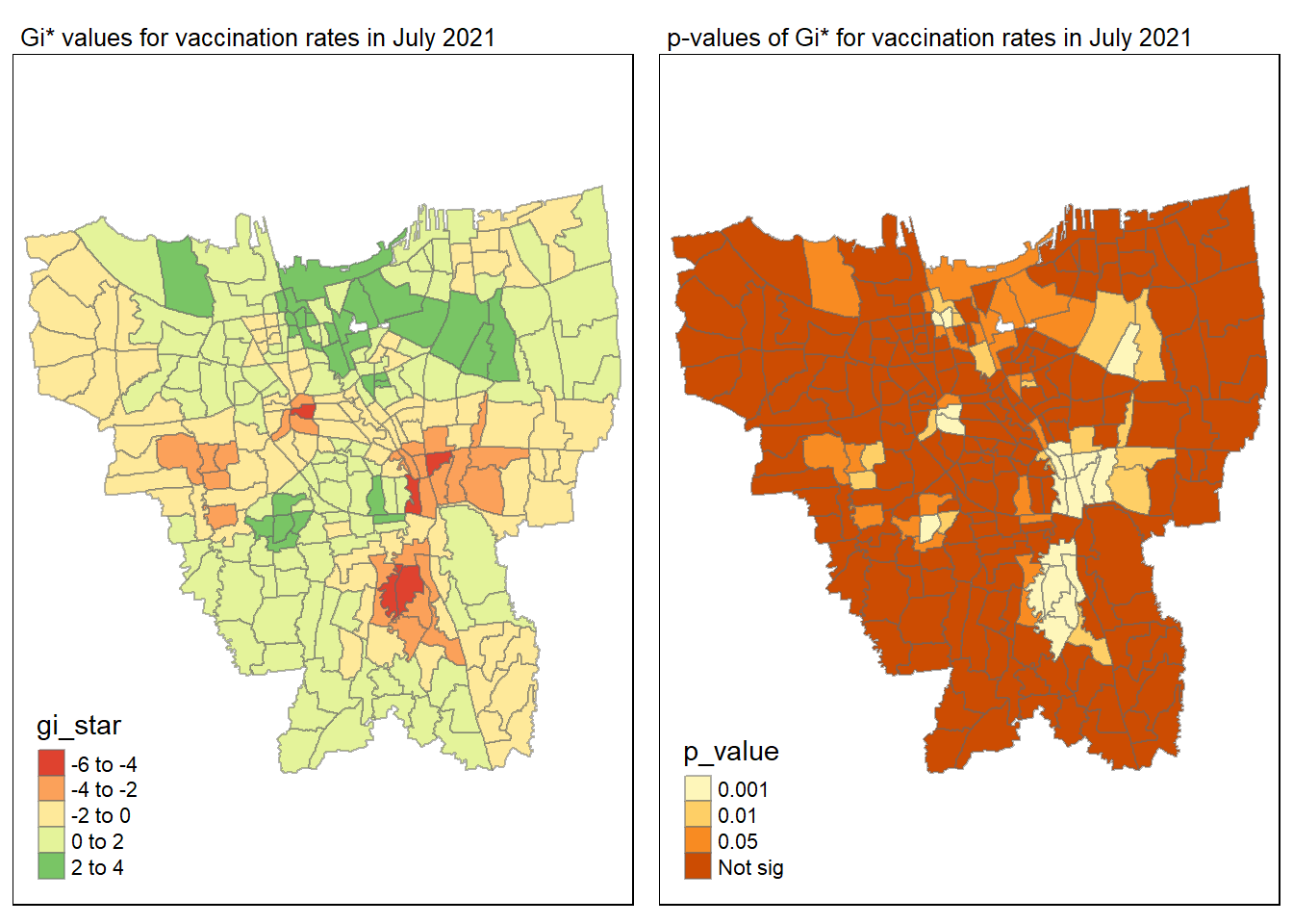

tmap_mode("plot")
gi_value_plot("2021-08-31", "August 2021")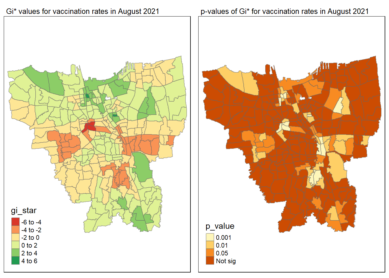

tmap_mode("plot")
gi_value_plot("2021-09-30", "September 2021")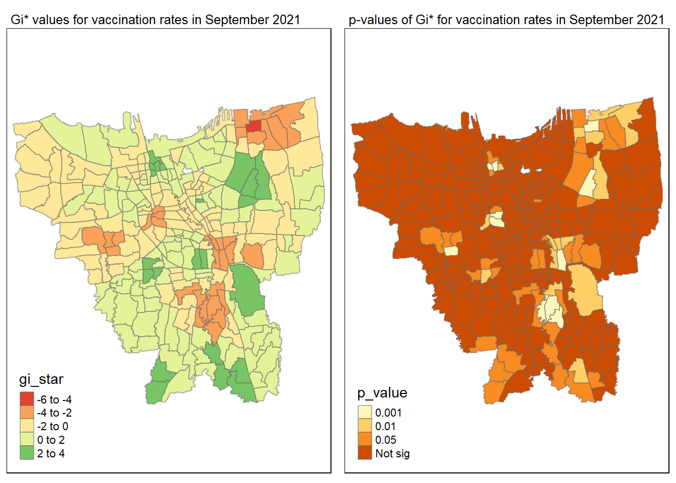

tmap_mode("plot")
gi_value_plot("2021-10-31", "October 2021")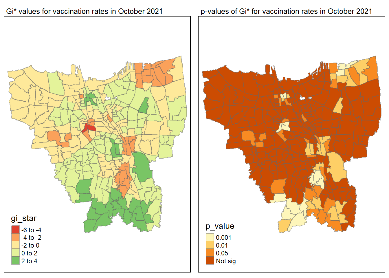

tmap_mode("plot")
gi_value_plot("2021-11-30", "November 2021")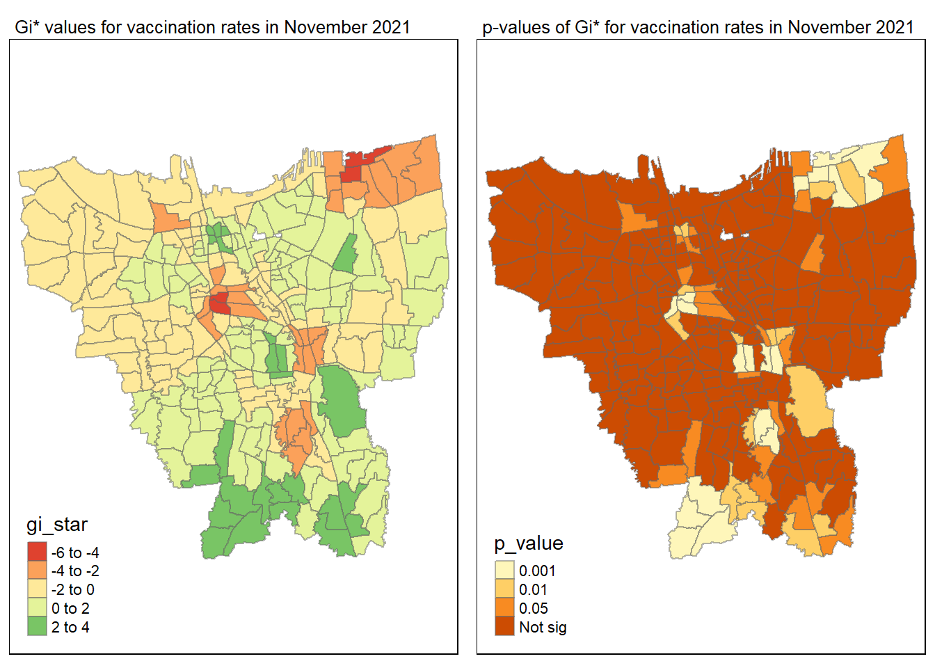

tmap_mode("plot")
gi_value_plot("2021-12-31", "December 2021")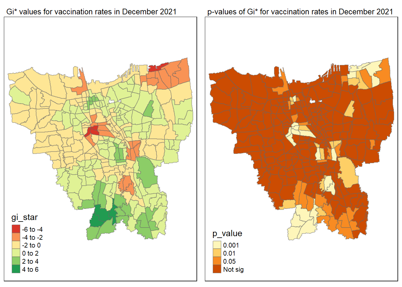

tmap_mode("plot")
gi_value_plot("2022-01-31", "January 2022")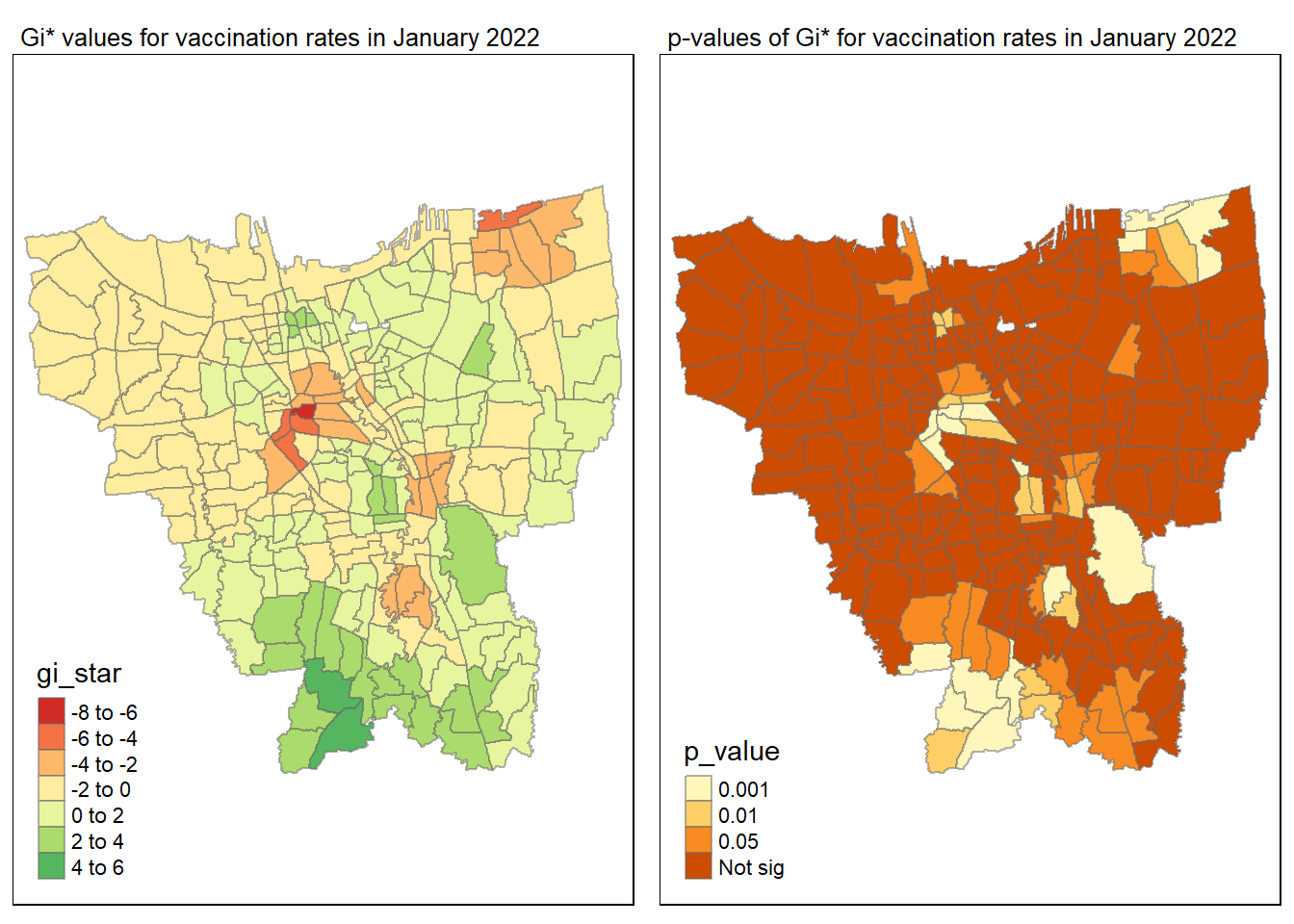

tmap_mode("plot")
gi_value_plot("2022-02-27", "February 2022")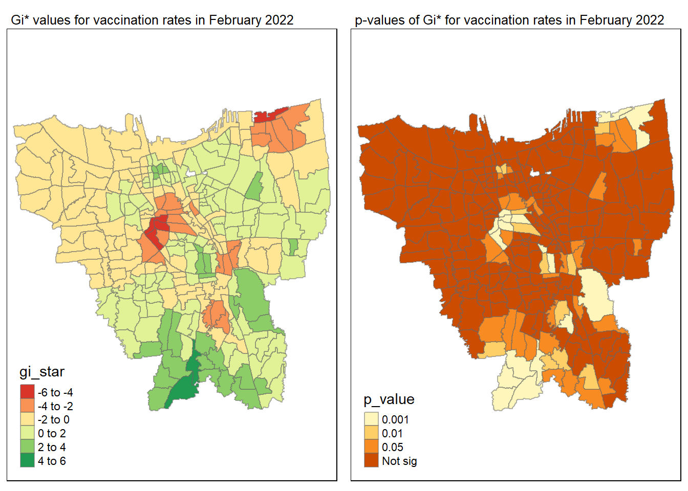

tmap_mode("plot")
gi_value_plot("2022-03-31", "March 2022")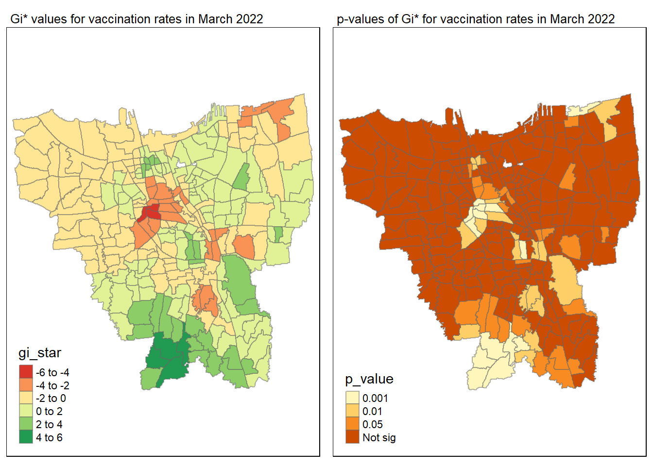

tmap_mode("plot")
gi_value_plot("2022-04-30", "April 2022")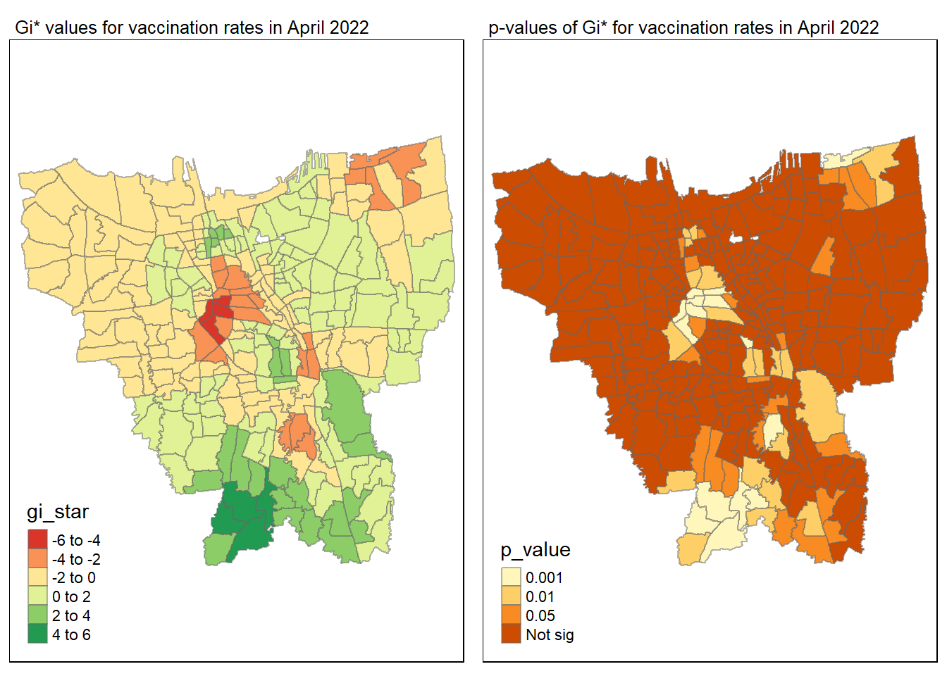

tmap_mode("plot")
gi_value_plot("2022-05-31", "May 2022")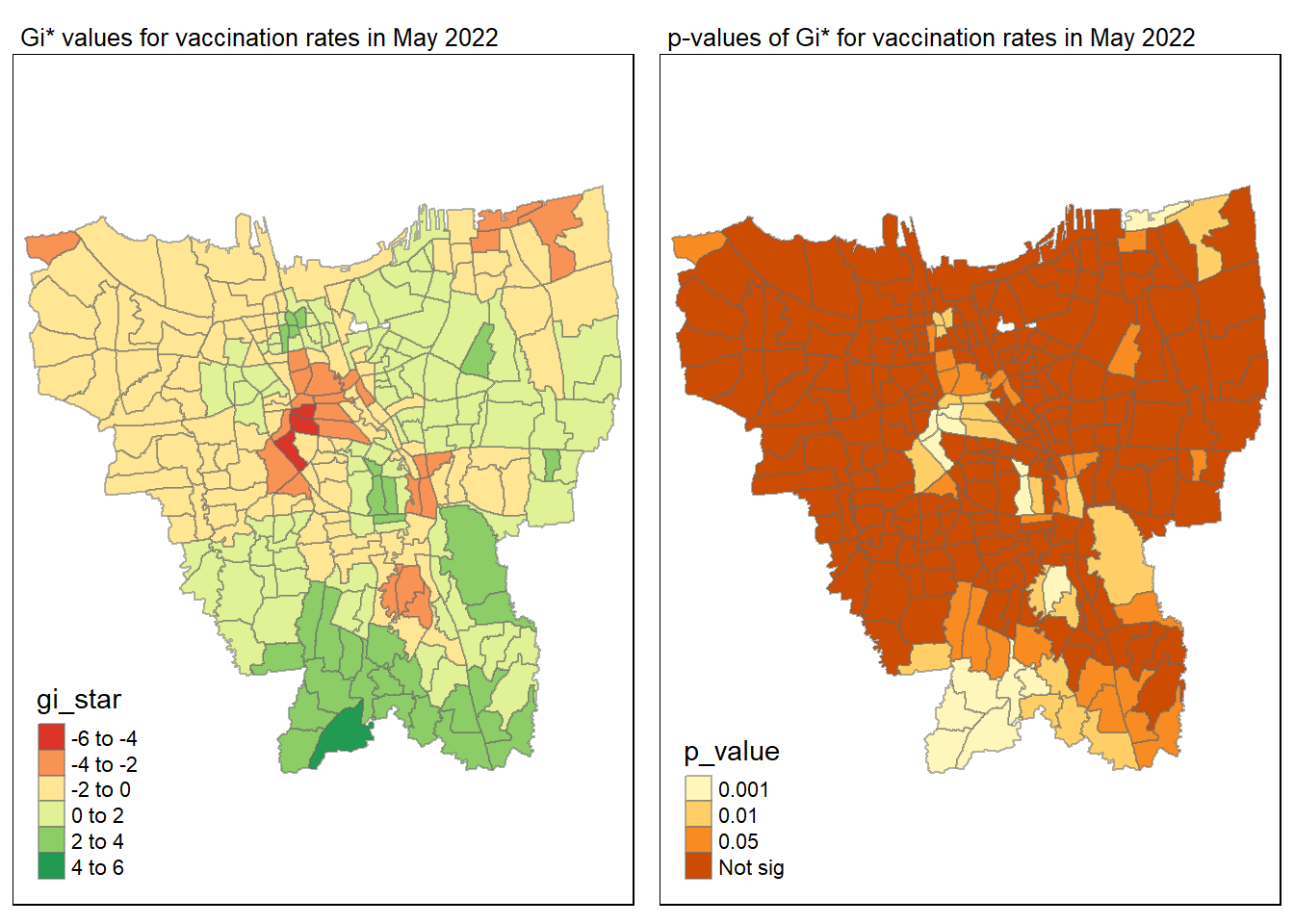

tmap_mode("plot")
gi_value_plot("2022-06-30", "June 2022")

Statistical conclusion

The p-value represents the probability of observing a clustering. A significant p-value < 0.05 suggests that an observed pattern is unlikely to have occurred by chance and may indicate the presence of a spatial process. When Gi* value > 0, it indicates sub-districts with a higher vaccination rate than average. We can view the number of sub districts with p-value < 0.05 with the code below

no_of_subdistricts_freq = filter(jakarta_gi_values, p_sim < 0.05)
as.data.frame(table(no_of_subdistricts_freq$Sub_District))

                      Var1 Freq
1                    ANCOL    1
2             BALE KAMBANG   11
3              BALI MESTER    4
4                     BARU    9
5               BATU AMPAR   12
6          BENDUNGAN HILIR   10
7              BIDARA CINA    9
8      CEMPAKA PUTIH BARAT    1
9                  CIBUBUR   10
10                CIGANJUR   10
11               CIJANTUNG   10
12                  CIKINI    1
13                  CIKOKO    8
14          CILANDAK BARAT    3
15          CILANDAK TIMUR    7
16               CILILITAN    4
17               CILINCING   10
18                CIPAYUNG    6
19                 CIPEDAK   10
20  CIPINANG BESAR SELATAN    3
21    CIPINANG BESAR UTARA    8
22       CIPINANG CEMPEDAK   12
23          CIPINANG MUARA    2
24                 CIPULIR    2
25                 CIRACAS    1
26             DUREN SAWIT    1
27            DURI SELATAN    1
28                   GALUR    2
29                  GAMBIR    5
30                  GEDONG    3
31                  GELORA    7
32                  GLODOK   12
33              GONDANGDIA    7
34          GROGOL SELATAN    1
35            GROGOL UTARA    1
36   GUNUNG SAHARI SELATAN    1
37     GUNUNG SAHARI UTARA    1
38   HALIM PERDANA KUSUMAH   11
39               JAGAKARSA    9
40              JATINEGARA    1
41         JATINEGARA KAUM    1
42           JEMBATAN LIMA    1
43              JOHAR BARU    1
44                KALIBARU   10
45                KALISARI    9
46                   KAMAL    1
47             KAMAL MUARA    1
48            KAMPUNG BALI   12
49          KAMPUNG MELAYU    3
50            KAMPUNG RAWA    3
51          KAMPUNG TENGAH   12
52             KAPUK MUARA    2
53           KARET TENGSIN    4
54              KAYU MANIS    1
55               KEAGUNGAN   12
56               KEBAGUSAN    5
57            KEBON KACANG   12
58            KEBON MELATI   12
59             KEBON SIRIH    7
60              KELAPA DUA    3
61        KELAPA DUA WETAN   11
62     KELAPA GADING BARAT    2
63     KELAPA GADING TIMUR    7
64                 KLENDER    2
65                    KOJA    2
66                  KRAMAT    2
67             KRAMAT JATI    3
68                   LAGOA    9
69           LENTENG AGUNG    9
70            LUBANG BUAYA    5
71             MALAKA JAYA    4
72             MALAKA SARI    1
73            MANGGA BESAR   12
74       MANGGARAI SELATAN    8
75                  MAPHAR    3
76                 MARUNDA    1
77                 MELAWAI    2
78                 MENTENG    7
79                  MUNJUL    9
80              PAL MERIAM    1
81                PAPANGGO    1
82              PASAR BARU    2
83           PASAR MANGGIS    2
84          PEGANGSAAN DUA    3
85           PEJATEN TIMUR    3
86                 PEKAYON    8
87            PENGGILINGAN    1
88             PENJARINGAN    2
89              PETAMBURAN   12
90               PETOGOGAN    2
91          PETOJO SELATAN    7
92            PETOJO UTARA    2
93        PETUKANGAN UTARA    1
94            PINANG RANTI    1
95               PINANGSIA    3
96           PISANGAN BARU    2
97          PISANGAN TIMUR    1
98            PONDOK BAMBU    4
99             PONDOK KOPI    2
100            PONDOK LABU    9
101            PULO GADUNG    2
102                RAGUNAN    7
103               RAMBUTAN    1
104     RAWA BADAK SELATAN    1
105       RAWA BADAK UTARA    4
106             RAWA BARAT    1
107             RAWA BUNGA    9
108             ROA MALAKA    1
109                 SELONG    2
110           SEMPER BARAT    5
111           SEMPER TIMUR    4
112                SENAYAN    2
113                  SENEN    2
114              SRENGSENG    1
115        SRENGSENG SAWAH    9
116       SUKABUMI SELATAN    4
117         SUKABUMI UTARA    3
118           SUNTER AGUNG    1
119            SUNTER JAYA    4
120           TANAH SEREAL    5
121           TANAH TINGGI    2
122                 TANGKI   10
123          TANJUNG BARAT    6
124            TEBET BARAT   10
125            TEBET TIMUR   10
126                 TOMANG    1
127             TUGU UTARA    5
128                ULUJAMI    1

From the table above, there are 128 sub-districts who have a significant vaccination rate p-value < 0.05 at least once during the period of 12 months. Those sub-districts that have double digits frequency have a significant p value throughout the entire 12 months.

7. Emerging Hot Spot Analysis (EHSA)

Emerging Hot Spot Analysis (EHSA) is a spatio-temporal analysis method for revealing and describing how hot spot and cold spot areas evolve over time. Previously we have already built a space-time cube and calculated the Gi. Therefore, we can directly conduct the Mann-Kendall trend test to evaluate 3 sub-districts for a trend. The 3 sub-districts chosen would be HALIM PERDANA KUSUMAH, TUGU UTARA and ULUJAMI.

7.1 Mann-Kendall Test

7.1.1 KEAGUNGAN

Keagungan <- gi_values |>
  ungroup() |>
  filter(Sub_District == "KEAGUNGAN") |>
  select(Sub_District, Date, gi_star)

Plotting the result by using ggplotly

p <- ggplot(data = Keagungan, 
       aes(x = Date, 
           y = gi_star)) +
  geom_line() +
  theme_light()

ggplotly(p)

Keagungan %>%
  summarise(mk = list(
    unclass(
      Kendall::MannKendall(gi_star)))) %>% 
  tidyr::unnest_wider(mk)

# A tibble: 1 x 5
    tau     sl     S     D  varS
  <dbl>  <dbl> <dbl> <dbl> <dbl>
1 0.455 0.0467    30  66.0  213.

The p-value is 0.046 which is < 0.05 hence p-value is significant. Therefore, this is a fluctuating upward significant trend.

7.1.2 HARAPAN MULIA

HARAPAN_MULIA <- gi_values |>
  ungroup() |>
  filter(Sub_District == "HARAPAN MULIA") |>
  select(Sub_District, Date, gi_star)

Plotting the result by using ggplotly

p <- ggplot(data = HARAPAN_MULIA, 
       aes(x = Date, 
           y = gi_star)) +
  geom_line() +
  theme_light()

ggplotly(p)

HARAPAN_MULIA %>%
  summarise(mk = list(
    unclass(
      Kendall::MannKendall(gi_star)))) %>% 
  tidyr::unnest_wider(mk)

# A tibble: 1 x 5
     tau    sl     S     D  varS
   <dbl> <dbl> <dbl> <dbl> <dbl>
1 0.0909 0.732     6  66.0  213.

The p-value is 0.73 which is > 0.05 hence p-value is not significant. Therefore, this is an downward insignificant trend.

7.1.3 ULUJAMI

ulujami <- gi_values |>
  ungroup() |>
  filter(Sub_District == "ULUJAMI") |>
  select(Sub_District, Date, gi_star)

Plotting the result by using ggplotly

p <- ggplot(data = ulujami, 
       aes(x = Date, 
           y = gi_star)) +
  geom_line() +
  theme_light()

ggplotly(p)

ulujami %>%
  summarise(mk = list(
    unclass(
      Kendall::MannKendall(gi_star)))) %>% 
  tidyr::unnest_wider(mk)

# A tibble: 1 x 5
    tau      sl     S     D  varS
  <dbl>   <dbl> <dbl> <dbl> <dbl>
1 0.667 0.00319    44  66.0  213.

The p-value is 0.003 which is < 0.05 hence p-value is significant. Therefore, this is an upward but significant trend.

7.2 EHSA map of the Gi* value

For us to find the significant hot and cold spots, there is a need to conduct the Mann Kendall test on all the subdistricts out there. Therefore, the group_by() function will be used for all subdistricts.

ehsa <- gi_values %>%
  group_by(Sub_District) %>%
  summarise(mk = list(
    unclass(
      Kendall::MannKendall(gi_star)))) %>%
  tidyr::unnest_wider(mk)

Show significant top 10 emerging hot/cold spots area

emerging <- ehsa %>% 
  arrange(sl, abs(tau)) %>% 
  slice(1:10)
emerging

# A tibble: 10 x 6
   Sub_District             tau        sl     S     D  varS
   <chr>                  <dbl>     <dbl> <dbl> <dbl> <dbl>
 1 PETOJO UTARA          -0.970 0.0000156   -64  66.0  213.
 2 KAYU MANIS             0.970 0.0000156    64  66.0  213.
 3 JATINEGARA KAUM        0.939 0.0000287    62  66.0  213.
 4 PISANGAN BARU          0.939 0.0000287    62  66.0  213.
 5 PASAR BARU            -0.939 0.0000288   -62  66.0  213.
 6 DUKUH                  0.909 0.0000521    60  66.0  213.
 7 KAMAL MUARA           -0.909 0.0000521   -60  66.0  213.
 8 KAPUK MUARA           -0.909 0.0000521   -60  66.0  213.
 9 KEBON KELAPA          -0.909 0.0000521   -60  66.0  213.
10 GUNUNG SAHARI SELATAN -0.879 0.0000928   -58  66.0  213.

emerging_hotspot_analysis() of sfdep package will be used to perform EHSA analysis. It takes a spacetime object x (i.e. vaccination_rate_st), and the quoted name of the variable of interest (i.e. Vaccinaton Rate) for .var argument. The k argument is used to specify the number of time lags which is set to 1 by default.

ehsa <- emerging_hotspot_analysis(
  x = vaccination_rate_st,
  .var = "Vaccination_Rate",
  k = 1,
  nsim = 99
)

Visualisation of distribution

ggplot(data = ehsa,
       aes(x=classification, fill=classification)) + 
  geom_bar()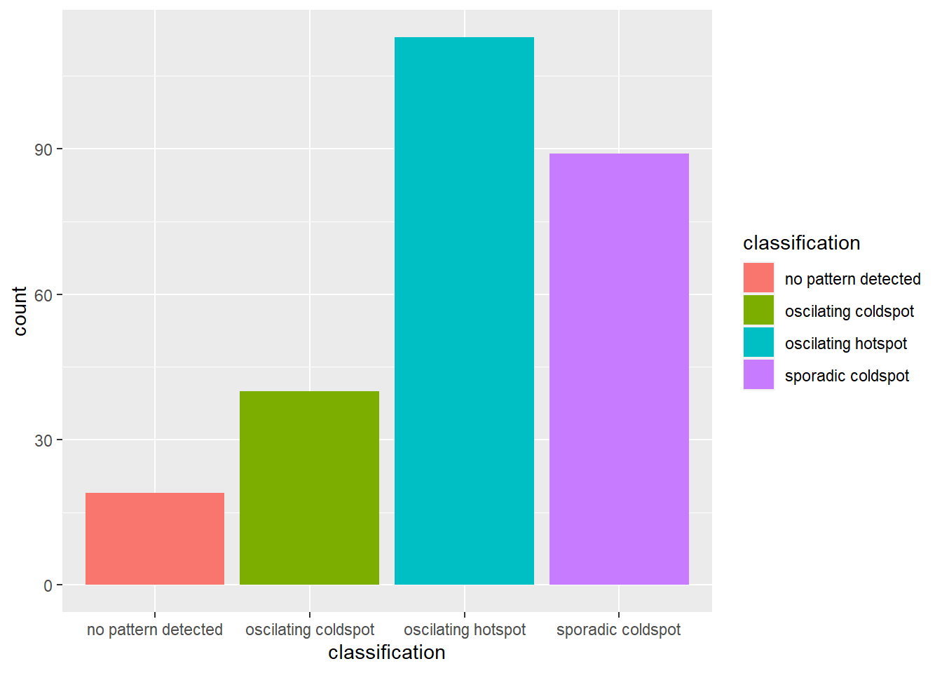

The barchart above shows that sporadic hot spots class has the highest numbers.

Left join of combine jakarta and ehsa together

jakarta_ehsa <- bd_jakarta %>%
  left_join(ehsa, by = c("Sub_District" = "location"))

Visualisation of classification using tmap

# We use the filter to filter out values with p-value < 0.05
jakarta_ehsa_sig <- jakarta_ehsa  %>%
  filter(p_value < 0.05)
tmap_mode("plot")
tm_shape(jakarta_ehsa) +
  tm_polygons() +
  tm_borders(alpha = 0.5) +
tm_shape(jakarta_ehsa_sig) +
  tm_fill("classification") + 
  tm_borders(alpha = 0.4)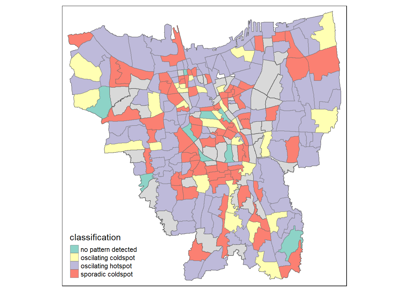

Observation:

Oscilating coldspot is spread out evenly in Jakarta which can be found to be more around the border and in the central of Jakarta. At the same time, the oscillating hotspot is lesser than spordiac coldspot. Similar to oscilating coldspot, there is also a large number of spordiac hotspot spread out evenly around Jakarta. From the map, the patterns are not obvious and the sub districts shaded in grey are of p value > 0.05 which means that the sub districts are insignificant.

End of take home exercise 2